Causal inference with beta regression

Sometimes in the methodological literature, models for continuous outcomes are presumed to use the Gaussian likelihood. In the sixth post of this series, we saw the gamma likelihood is a great alternative when your continuous data are restricted to positive values, such as in reaction times and bodyweight. In this ninth post, we practice making causal inferences with the beta likelihood for continuous data restricted within the range of \((0, 1)\).

Reload the data

In this post, we’ll be continuing on with our hoorelbeke2021 data set from the last post on change scores. These data, recall, come from Hoorelbeke et al. ( 2021), who saved them in a Baseline & FU rating.sav file uploaded to the OSF at https://osf.io/6ptu5/. ⚠️ For this next code block to work on your computer, you will need to first download that Baseline & FU rating.sav file, and then save that file in a data subfolder in your working directory.

# packages
library(tidyverse)
library(brms)
library(patchwork)
library(tidybayes)
library(marginaleffects)

# adjust the global theme
theme_set(theme_gray(base_size = 12) +
            theme(panel.grid = element_blank()))

# load the data
hoorelbeke2021 <- haven::read_sav("data/Baseline & FU rating.sav")

# wrangle
hoorelbeke2021 <- hoorelbeke2021 %>% 
  drop_na(Acc_naPASAT_FollowUp) %>% 
  transmute(id     = ID,
            tx     = Group,
            pre    = Acc_naPASAT_Baseline,
            post   = Acc_naPASAT_FollowUp,
            change = Acc_naPASAT_FollowUp - Acc_naPASAT_Baseline)

# what?
glimpse(hoorelbeke2021)

## Rows: 82
## Columns: 5
## $ id     <dbl> 1, 2, 3, 4, 5, 6, 7, 8, 9, 10, 11, 12, 13, 14, 16, 17, 18, 19, 20, 21, 22, 24, 25, 26, 27, 28…
## $ tx     <dbl> 1, 0, 1, 0, 1, 0, 1, 0, 1, 0, 1, 0, 1, 0, 0, 1, 0, 1, 0, 1, 0, 0, 1, 0, 1, 0, 1, 0, 1, 1, 1, …
## $ pre    <dbl> 0.3444444, 0.5111111, 0.5833333, 0.6444444, 0.6944444, 0.3388889, 0.7833333, 0.5888889, 0.738…
## $ post   <dbl> 0.9166667, 0.7000000, 0.8166667, 0.7722222, 0.9000000, 0.3888889, 0.9833333, 0.6944444, 0.972…
## $ change <dbl> 0.57222222, 0.18888889, 0.23333333, 0.12777778, 0.20555556, 0.05000000, 0.20000000, 0.1055555…

We’re not going to go into a full introduction of these data, again. You have the last post for that. But I do think we should warm up with another exploratory plot. This time, we’ll make scatter plots with pre on the \(x\) and post on the \(y\), separated by the two levels of the experimental grouping variable tx.

hoorelbeke2021 %>% 
  ggplot(aes(x = pre, y = post)) +
  geom_hline(yintercept = 0:1, color = "white") +
  geom_vline(xintercept = 0:1, color = "white") +
  geom_abline(color = "white") +
  stat_smooth(method = "lm", formula = 'y ~ x', se = F) +
  geom_point() +
  scale_x_continuous(breaks = 0:5 / 5) +
  scale_y_continuous(breaks = 0:5 / 5) +
  coord_equal(xlim = 0:1,
              ylim = 0:1) +
  facet_wrap(~ tx, labeller = label_both)

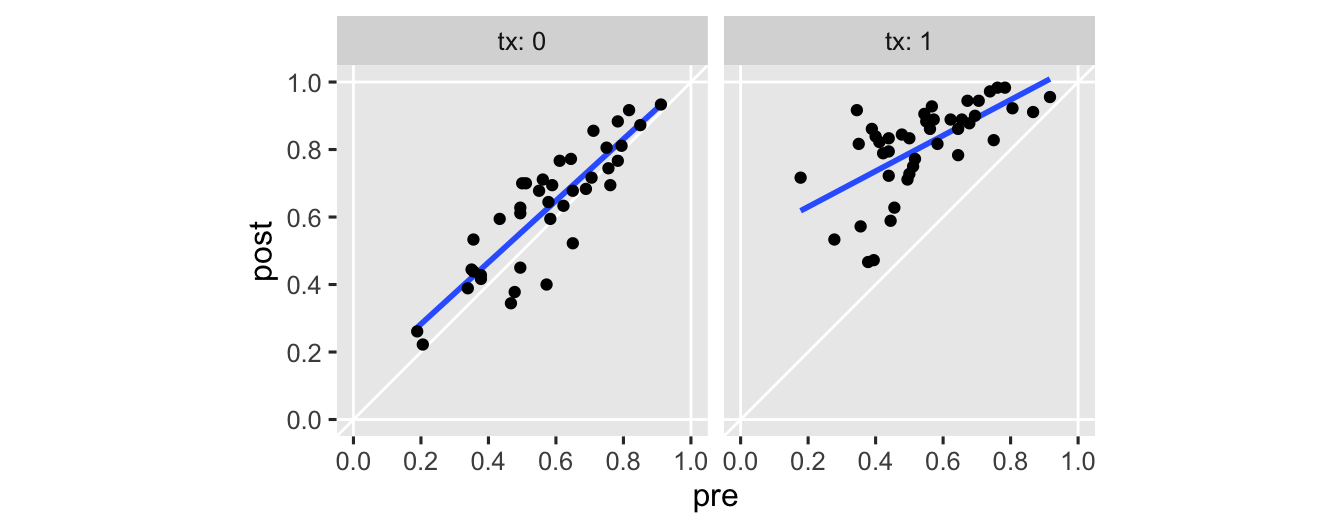
Note the vertical and horizontal white lines at the edges of the panels mark off the \((0, 1)\) boundaries for both axes. The OLS fitted lines are in blue. There’s nothing keeping a conventional OLS (i.e., Gaussian) model from crossing those boundaries, which you see in the upper right of the panel in the right. It’s subtle, but you might also notice how the data tend to show less scatter as they approach the upper limit. That’s heteroskedasticity, friends, and it’s also not a great fit for a conventional Gaussian model.

Model framework

It’s possible to fit beta regression models in R with packages like betareg ( Cribari-Neto & Zeileis, 2010; Grün et al., 2012; Zeileis et al., 2021) and glmmTMB ( M. Brooks et al., 2023; M. E. Brooks et al., 2017). Here we’re just going to jump straight into Bayesland and fit our models with brms. Before we fit the beta models, though, we’ll warm up with the Gauss. Using both likelihoods, we’ll analyze the data with an ANOVA and an ANCOVA, which will make for 4 models in total.

Normal Gaussian models.

If we ignore the data boundaries and the heteroskedasticity issue, we might fit a simple Bayesian Gaussian ANOVA of the form

$$ \begin{align*} \text{post}_i & \sim \operatorname{Normal}(\mu_i, \sigma) \\ \mu_i & = \beta_0 + \beta_1 \text{tx}_i \\ \beta_0 & \sim \operatorname{Normal}(0.5, 0.2) \\ \beta_1 & \sim \operatorname{Normal}(0, 0.2) \\ \sigma & \sim \operatorname{Exponential}(4), \end{align*} $$

where the intercept \(\beta_0\) is the mean for those in the control condition, the slope \(\beta_1\) is the difference in means for those in the experimental condition, and \(\sigma\) denotes the residual standard deviation in post values. The last three lines are our priors, which we’ll explain in order below.

Whenever I’m setting an intercept prior for data with lower and upper boundaries, I typically default to the mean of the distribution. Since our post range between 0 and 1, 0.5 seems like a great place to center our prior for \(\beta_0\). However, I’m not an aPASAT researcher, and thus if you were and you had a better sense of what a typical average value was for the aPASAT, you could very rightly use that in place of my 0.5. Given the scale of the data, the 0.2 hyperparameter for the scale of the \(\beta_0\) prior is meant to be weakly regularizing. To give you a sense, here’s a plot of the prior.

prior(normal(0.5, 0.2)) %>% 
  parse_dist() %>% 
  
  ggplot(aes(xdist = .dist_obj, y = prior)) + 
  stat_halfeye(.width = c(.5, .99)) +
  scale_x_continuous(expression(italic(p)(beta[0])), breaks = 0:10 / 10) +
  scale_y_discrete(NULL, breaks = NULL, expand = expansion(add = 0.1)) +
  coord_cartesian(xlim = c(0, 1))

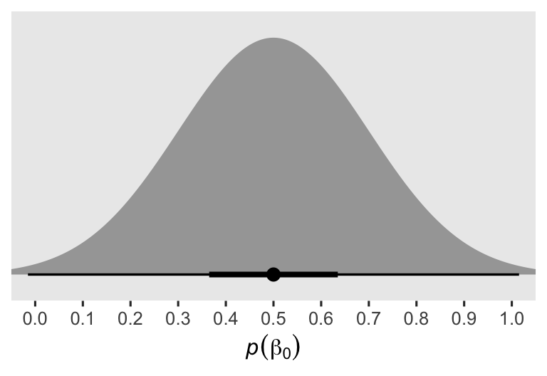
Though the interquartile range is within 0.36 and 0.64, the 99% range extends just beyond the logical 0 and 1 boundaries. The prior is gentle, and a well-informed substantive researcher could probably do much better, and justify a tighter prior standard deviation.

The \(\operatorname{Normal}(0, 0.2)\) prior for \(\beta_1\) is meant to be weakly regularizing. It will allow for small to large group differences, but rule out the outrageously large. As is often the case for parameters like this, I’ve centered the prior on 0 to encourage slightly conservative results.

Given the data are constrained between 0 and 1, the maximum standard deviation possible is 0.5.¹ Here’s a quick proof:

sd(rep(0:1, each = 1e6))

## [1] 0.5000001

But since this is the maximum value, I wanted a prior centered closer to zero. The exponential distribution, recall, is parameterized in terms of the single value \(\lambda\), which is the inverse of the mean. Thus an \(\operatorname{Exponential}(4)\) has a mean of 0.25, the lower half of the prior mass ranges between 0 and 0.25, and the rest of the prior mass gradually tapers to the right. A well-informed substantive researcher could no doubt pick a better prior for \(\sigma\), but this seems like a good place to start.

Expanding, we might define our Bayesian Gaussian ANCOVA as

$$ \begin{align*} \text{post}_i & \sim \operatorname{Normal}(\mu_i, \sigma) \\ \mu_i & = \beta_0 + \beta_1 \text{tx}_i + \beta_2 \text{prec}_i \\ \beta_0 & \sim \operatorname{Normal}(0.5, 0.2) \\ \beta_1 & \sim \operatorname{Normal}(0, 0.2) \\ \beta_2 & \sim \operatorname{Normal}(1, 0.2) \\ \sigma & \sim \operatorname{Exponential}(4), \end{align*} $$

where the new parameter \(\beta_2\) controls for the mean-centered version of the baseline aPASAT scores pre. Before we forget, we should probably add that prec variable to the data set.

hoorelbeke2021 <- hoorelbeke2021 %>% 
  mutate(txf = factor(tx)) %>% 
  mutate(prec = pre - mean(pre))

# what?
hoorelbeke2021 %>% 
  select(pre, prec) %>% 
  head()

## # A tibble: 6 × 2
##     pre    prec
##   <dbl>   <dbl>
## 1 0.344 -0.214 
## 2 0.511 -0.0472
## 3 0.583  0.0251
## 4 0.644  0.0862
## 5 0.694  0.136 
## 6 0.339 -0.219

Centering the prior on \(\beta_2\) on 1 optimistically expresses my expectation baseline aPASAT would have a strong positive correlation with posttest aPASAT scores. Less enthusiastic modelers might use something like \(\operatorname{Normal}(0.5, 0.2)\) instead.

Before we fit the models, you might also note we saved a factor version of the tx dummy as txf. This usually isn’t necessary, but it will help with the pp_check() plots later on.

Here’s how to fit the Gaussian ANOVA and ANCOVA models with brm().

# Gaussian ANOVA
fit1g <- brm(
  data = hoorelbeke2021,
  family = gaussian,
  post ~ 0 + Intercept + txf,
  prior = prior(normal(0.5, 0.2), class = b, coef = Intercept) +
    prior(normal(0, 0.2), class = b, coef = txf1) +
    prior(exponential(4), class = sigma),
  cores = 4, seed = 9
)

# Gaussian ANCOVA
fit2g <- brm(
  data = hoorelbeke2021,
  family = gaussian,
  post ~ 0 + Intercept + txf + prec,
  prior = prior(normal(0.5, 0.2), class = b, coef = Intercept) +
    prior(normal(0, 0.2), class = b, coef = txf1) +
    prior(normal(1, 0.2), class = b, coef = prec) +
    prior(exponential(4), class = sigma),
  cores = 4, seed = 9
)

As a reminder, we’re using the 0 + Intercept + ... syntax because both models contain at least one predictor variable, txf, that is not mean centered.²

Since these are pretty simple Bayesian models, I’m not going to clutter up the blog post with their print() output. But if you’re following along on your computer, I recommend executing the code below to review the output. In short, the model summaries look fine.

print(fit1g)
print(fit2g)

Beta likelihood.

So far in this blog series, our models have been housed within the generalized linear model (GLM) paradigm. The GLM has its origins in Nelder & Wedderburn ( 1972), and it includes models with likelihood functions from the exponential family, such as the Gaussian, Poisson, and binomial.³ The beta likelihood, however, is not typically considered as part of the exponential family, and therefore not a candidate for the GLM.⁴ Thus even though this post is part of my GLM and causal inference series, we’re using the term GLM in a lose nontraditional sense, here. I suppose you could say we’re referring to beta regression as a “GLM” in scare quotes more so than a GLM.⁵ Had my foresight been better, maybe I would have chosen a different name for this series. So it goes…

Anyway, to my knowledge the beta-regression model was first proposed by Paolino ( 2001). Sometimes Ferrari & Cribari-Neto ( 2004) is listed as the first paper, and it’s a fine paper, but it clearly came later than Paolino ( 2001). Since then, numerous scholars have proposed nice generalizations, which we’ll briefly discuss at the end of the post. For most of this blog post, though, our beta-regression models will be of simple kind.

Given some continuous variable \(y\) which is constrained to the range \((0, 1)\), the canonical parameterization for the beta likelihood is

$$ f(y | \alpha, \beta) = \frac{y^{\alpha - 1 } (1 - y)^{\beta - 1}}{\operatorname{B}(\alpha, \beta)}, $$

where \(\operatorname{B}(\cdot)\) is the beta function, and the two free parameters in the likelihood are \(\alpha\) and \(\beta\). With this parameterization, the mean of the population distribution will be

$$\mathbb E(y) = \frac{\alpha}{\alpha + \beta},$$

and the variance will be

$$ \operatorname{Var}(y) = \frac{\alpha \beta}{(\alpha + \beta)^2 (\alpha + \beta + 1)}. $$

Notice how the formulas for the mean and variance both contain the sum \(\alpha + \beta\). This quantity is sometimes called the concentration, sample size or precision, and it is often denoted with the Greek symbols \(\nu\) or \(\kappa\). The idea of sample size comes from the shape the binomial likelihood can take for \(p\) given \(\alpha\) \(1\)’s out of \(\alpha + \beta\) Bernoulli trials. Thus, smaller values for the concentration/precision/sample size make for wider distributions, whereas larger values make for narrower distributions. Thus, larger values result in a more concentrated density around the mean.

The canonical parameterization is limited in it does not lend itself well to the regression framework. Happily, we can also express the beta distribution in terms of its mean and concentration. Using the brms notation ( Bürkner, 2023c), this looks like

$$ f(y | \mu, \phi) = \frac{y^{\mu \phi - 1 } (1 - y)^{(1 - \mu)\phi - 1}}{\operatorname{B}(\mu \phi, [1 - \mu]\phi)}, $$

where we refer to the mean as \(\mu\) and the concentration as \(\phi\). But do note that whereas brms uses the notation of \(\phi\) and the language of precision, this is the same value we also often call \(\nu\) or \(\kappa\). If desired, we can connect this parameterization to the canonical parameterization with the formulas

$$ \begin{align*} \alpha & = \mu \phi, \text{and} \\ \beta & = (1 - \mu)\phi. \end{align*} $$

To bring this all down to Earth, let’s see what this looks like in the context of a couple models. I propose we fit our beta-regression version of the ANOVA with the equation

$$ \begin{align*} \text{post}_i & \sim \operatorname{Beta}(\mu_i, \phi) \\ \operatorname{logit}(\mu_i) & = \beta_0 + \beta_1 \text{tx}_i \\ \beta_0, \beta_1 & \sim \operatorname{Normal}(0, 1) \\ \phi & \sim \operatorname{Gamma}(4, 0.1), \end{align*} $$

where the first line indicates we’re using the \(\mu\) and \(\phi\) parameterization for beta. The left-hand side of the second line shows we’re using the logit link to ensure the \(\mu_i\) model will only predict mean values for beta within the \((0, 1)\) range, much like we do with a logistic regression model for binary data. If you wanted to, I suppose you could use an alternative link like the probit, instead. But since we’re using the brm() default logit link, it’s important to understand that will put the \(\beta\) parameters on the log-odds scale. Speaking of which, the third and fourth lines in the equation define the priors for our parameters, which we’ll detail next.

When I fit Bayesian logistic regression models, \(\operatorname{Normal}(0, 1)\) is my default weakly-regularizing prior, and I think it’s a good default for beta regression too. When we use this prior for \(\beta_0\), we’re suggesting the mean aPASAT score for those on the control group should be around, 0.5, but with considerable uncertainty. To give you a sense, here we’ll simulate from the \(\operatorname{Normal}(0, 1)\) on the log-odds scale, and then use the plogis() function to convert the results back to the natural metric for the beta distribution.

set.seed(9)

tibble(lo = rnorm(n = 1e6, mean = 0, sd = 1)) %>% 
  mutate(b = plogis(lo)) %>% 
  pivot_longer(everything(), names_to = "metric") %>% 
  mutate(metric = ifelse(metric == "lo", "log odds", "beta") %>% 
           factor(levels = c("log odds", "beta"))) %>% 
  
  ggplot(aes(x = value)) +
  geom_histogram(boundary = 0, fill = "grey67") +
  stat_pointinterval(.width = c(.5, .99)) +
  scale_y_continuous(NULL, breaks = NULL) +
  labs(title = "Beta ANOVA",
       x = expression(italic(p)(beta[0]))) +
  facet_wrap(~ metric, scales = "free", labeller = label_both)

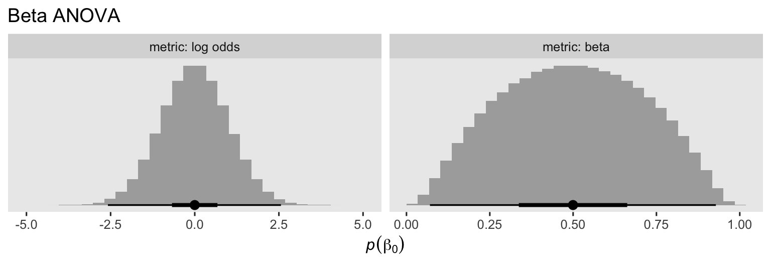
Thus the \(\operatorname{Normal}(0, 1)\) prior for \(\beta_0\) on the log-odds scale isn’t identical to the \(\operatorname{Normal}(0.5, 0.2)\) prior for \(\beta_0\) we used for the Gaussian ANOVA, but they’re pretty similar, particularly for the mean and interquartile range.

As to \(\beta_1\), the \(\operatorname{Normal}(0, 1)\) will allow for small to large group differences on the log-odds scale, but rule out the outrageously large.

We’ll need to do a little work to understand our \(\operatorname{Gamma}(4, 0.1)\) prior for \(\phi\). Earlier we described \(\phi\) as a precision parameter. \(\phi\) can take on positive real values, and larger values mean greater concentration around the mean–hence greater precision. To give a sense, we’ll plot the shapes for several different combinations of \(\mu\) and \(\phi\).

crossing(mu = c(.5, .75, .9),
         phi = c(0.1, 1, 10, 100)) %>% 
  expand(nesting(mu, phi),
         beta = seq(from = .001, to = .999, length.out = 300)) %>% 
  mutate(d   = dbeta(beta, shape1 = mu * phi, shape2 = phi - (mu * phi)),
         mu  = str_c("mu==", mu),
         phi = str_c("phi==", phi)) %>% 
  mutate(phi = factor(phi, levels = str_c("phi==", c(0.1, 1, 10, 100)))) %>% 
  
  ggplot(aes(x = beta, y = d)) +
  geom_area() +
  scale_x_continuous(breaks = 0:2 / 2, labels = c("0", ".5", "1")) +
  scale_y_continuous("density", breaks = NULL) +
  ggtitle(expression("Beta given different combinations of "*mu*" and "*phi)) +
  coord_cartesian(ylim = c(0, 14)) +
  facet_grid(mu ~ phi, labeller = label_parsed) +
  theme(panel.grid = element_blank())

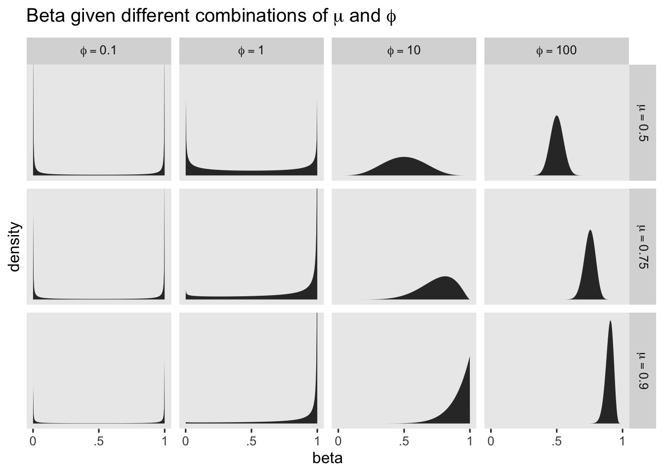
The beta distribution can take on odd-looking bimodal shapes when \(\phi\) approaches zero, which doesn’t seem like a great fit for us. But once \(\phi\) get’s into the double digits, the beta distribution takes on shapes that look a lot like what I would expect from the kind of data we tend to collect in clinical psychology. Thus to my mind, even if you and I aren’t expert aPASAT researchers, I think we want a prior for \(\phi\) that’s constrained to positive real values, and is concentrated primarily in the double-digit range. The brm() default prior for \(\phi\) is \(\operatorname{Gamma}(0.01, 0.01)\), and we’ll plot that in just a bit. We’ll take a cue from the brm() default and use a gamma prior, but with different hyperparameters. Here’s a plot of both.

c(prior(gamma(0.01, 0.01)),  # brms default
  prior(gamma(4, 0.1))) %>%  # Solomon's alternative
  parse_dist() %>% 
  
  ggplot(aes(xdist = .dist_obj, y = prior)) + 
  stat_halfeye(.width = c(.5, .99), p_limits = c(.0001, .9999)) +
  scale_x_continuous(expression(italic(p)(phi)), breaks = 0:4 * 25) +
  scale_y_discrete(NULL, expand = expansion(add = 0.1)) +
  labs(title = "Beta ANOVA") +
  coord_cartesian(xlim = c(0, 110))

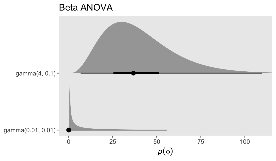
If you haven’t seen it before, the brm() default \(\operatorname{Gamma}(0.01, 0.01)\) has an odd-looking L shape, but my experience is it tends to work remarkably well when you don’t know where to start. Try it out for yourself and see. But since we’re in the 9th post of this series, it seems like it’s time to graduate past defaults. The bulk of the mass of our theory-based \(\operatorname{Gamma}(4, 0.1)\) prior is concentrated in the double-digit range. It has a mean of 40, a standard deviation of 20, an interquartile range of about 25 to 50, and a long right tail that will allow for greater concentrations if needed. You should feel free to play around with other priors for \(\phi\), but this one seems pretty good to me.⁶

Expanding, we might define our Bayesian beta ANCOVA as

$$ \begin{align*} \text{post}_i & \sim \operatorname{Beta}(\mu_i, \phi) \\ \operatorname{logit}(\mu_i) & = \beta_0 + \beta_1 \text{tx}_i + \beta_2 \text{prelo}_i \\ \beta_0, \beta_1 & \sim \operatorname{Normal}(0, 1) \\ \beta_2 & \sim \operatorname{Normal}(1, 1) \\ \phi & \sim \operatorname{Gamma}(4, 0.1), \end{align*} $$

where the new parameter \(\beta_2\) controls for the log-odds transformed version of the baseline aPASAT scores pre. Before we forget, we should probably add that prelo variable to the data set.

hoorelbeke2021 <- hoorelbeke2021 %>% 
  # qlogis() transforms (0, 1) values to the log-odds scale
  mutate(prelo = qlogis(pre))

# what?
hoorelbeke2021 %>% 
  select(pre, prec, prelo) %>% 
  head()

## # A tibble: 6 × 3
##     pre    prec   prelo
##   <dbl>   <dbl>   <dbl>
## 1 0.344 -0.214  -0.644 
## 2 0.511 -0.0472  0.0445
## 3 0.583  0.0251  0.336 
## 4 0.644  0.0862  0.595 
## 5 0.694  0.136   0.821 
## 6 0.339 -0.219  -0.668

Technically, we didn’t have to transform pre to the log-odds metric. But since we’re already modeling the mean of post on the log-odds, I think it makes sense to assume the log-odds version of pre would have the nicest conditional linear relation. To get a sense, here what the log-odds of both variables look like in an exploratory plot.

hoorelbeke2021 %>% 
  ggplot(aes(x = qlogis(pre), y = qlogis(post))) +
  geom_abline(color = "white") +
  geom_point() +
  coord_equal(xlim = c(-4, 4),
              ylim = c(-4, 4)) +
  labs(subtitle = "This looks linear, to me.") +
  facet_wrap(~ tx, labeller = label_both)

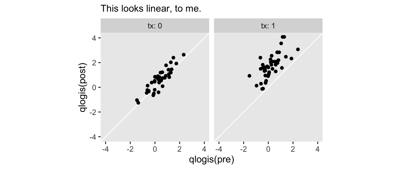
With this parameterization, the \(\operatorname{Normal}(1, 1)\) prior for \(\beta_2\) is designed to play a similar role as the \(\operatorname{Normal}(1, 0.2)\) we used back the Gaussian version of the model. It optimistically expresses my expectation baseline aPASAT would have a strong positive correlation with posttest aPASAT scores.

Okay, that’s been a lot of exposition. Here’s how to actually fit those beta models with the brm() function. Note how you use a capital “B” when setting family = Beta within brm(). If you don’t, you’ll get an error. By default, brm() assumes you want the logit link for the \(\mu_i\) model, and it presumes you want the identity link for \(\phi\).

# beta ANOVA
fit1b <- brm(
  data = hoorelbeke2021,
  family = Beta,
  post ~ 0 + Intercept + txf,
  prior = prior(normal(0, 1), class = b) +
    prior(gamma(4, 0.1), class = phi),
  cores = 4, seed = 9
)

# beta ANCOVA
fit2b <- brm(
  data = hoorelbeke2021,
  family = Beta,
  post ~ 0 + Intercept + txf + prelo,
  prior = prior(normal(0, 1), class = b) +
    prior(normal(1, 1), class = b, coef = prelo) +
    prior(gamma(4, 0.1), class = phi),
  cores = 4, seed = 9
)

Since we’re new to beta regression models, it’s probably worth your time to look over the print() output.

print(fit1b)  # beta ANOVA

##  Family: beta 
##   Links: mu = logit; phi = identity 
## Formula: post ~ 0 + Intercept + txf 
##    Data: hoorelbeke2021 (Number of observations: 82) 
##   Draws: 4 chains, each with iter = 2000; warmup = 1000; thin = 1;
##          total post-warmup draws = 4000
## 
## Population-Level Effects: 
##           Estimate Est.Error l-95% CI u-95% CI Rhat Bulk_ESS Tail_ESS
## Intercept     0.52      0.11     0.30     0.73 1.00     2103     2587
## txf1          0.90      0.16     0.59     1.21 1.00     2325     2562
## 
## Family Specific Parameters: 
##     Estimate Est.Error l-95% CI u-95% CI Rhat Bulk_ESS Tail_ESS
## phi     7.71      1.11     5.77    10.04 1.00     2497     2425
## 
## Draws were sampled using sampling(NUTS). For each parameter, Bulk_ESS
## and Tail_ESS are effective sample size measures, and Rhat is the potential
## scale reduction factor on split chains (at convergence, Rhat = 1).

print(fit2b)  # beta ANCOVA

##  Family: beta 
##   Links: mu = logit; phi = identity 
## Formula: post ~ 0 + Intercept + txf + prelo 
##    Data: hoorelbeke2021 (Number of observations: 82) 
##   Draws: 4 chains, each with iter = 2000; warmup = 1000; thin = 1;
##          total post-warmup draws = 4000
## 
## Population-Level Effects: 
##           Estimate Est.Error l-95% CI u-95% CI Rhat Bulk_ESS Tail_ESS
## Intercept     0.27      0.08     0.12     0.42 1.00     2855     2762
## txf1          1.13      0.11     0.90     1.35 1.00     2762     2355
## prelo         0.85      0.08     0.70     1.01 1.00     2905     2414
## 
## Family Specific Parameters: 
##     Estimate Est.Error l-95% CI u-95% CI Rhat Bulk_ESS Tail_ESS
## phi    20.59      3.04    15.10    26.98 1.00     2970     2425
## 
## Draws were sampled using sampling(NUTS). For each parameter, Bulk_ESS
## and Tail_ESS are effective sample size measures, and Rhat is the potential
## scale reduction factor on split chains (at convergence, Rhat = 1).

Turns out the \(\phi\) posteriors are on the low end of what I anticipated with those \(\operatorname{Gamma}(4, 0.1)\) priors. That’s okay, though. Priors aren’t supposed to be perfect. They’re supposed to convey your assumptions about the model, before you actually fit the model.

Posterior predictive checks.

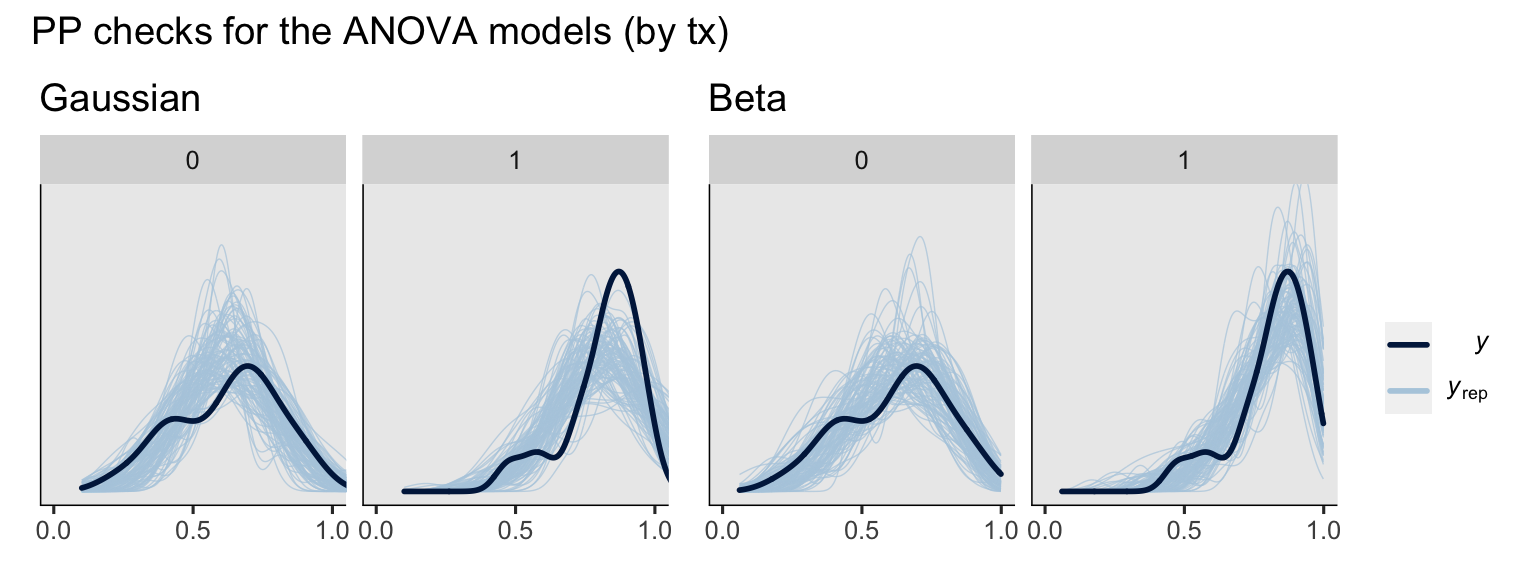
Before we dive into the potential outcomes and causal estimands, we might compare the overall predictive performance of the two likelihoods. I’m not going to compare the Gaussian and beta models with information criteria contrasts, because my understanding is it’s not the best idea to compare models with radically different likelihood functions in that way (see McElreath, 2020). We can, however, compare the models with a few posterior predictive checks. To start, we’ll make a few grouped density-overlay plots.

# ANOVA's
set.seed(9)
p1 <- pp_check(fit1g, type = "dens_overlay_grouped", group = "txf", ndraws = 100) +
  ggtitle("Gaussian") +
  scale_x_continuous(breaks = 0:2 / 2) +
  coord_cartesian(xlim = 0:1,
                  ylim = c(0, 5))

set.seed(9)
p2 <- pp_check(fit1b, type = "dens_overlay_grouped", group = "txf", ndraws = 100) +
  ggtitle("Beta") +
  scale_x_continuous(breaks = 0:2 / 2) +
  coord_cartesian(xlim = 0:1,
                  ylim = c(0, 5))

# ANCOVA's
set.seed(9)
p3 <- pp_check(fit2g, type = "dens_overlay_grouped", group = "txf", ndraws = 100) +
  ggtitle("Gaussian") +
  scale_x_continuous(breaks = 0:2 / 2) +
  coord_cartesian(xlim = 0:1,
                  ylim = c(0, 5))

set.seed(9)
p4 <- pp_check(fit2b, type = "dens_overlay_grouped", group = "txf", ndraws = 100) +
  ggtitle("Beta") +
  scale_x_continuous(breaks = 0:2 / 2) +
  coord_cartesian(xlim = 0:1,
                  ylim = c(0, 5))

# combine ANOVA's
p1 + p2 + 
  plot_layout(guides = "collect") +
  plot_annotation(title = "PP checks for the ANOVA models (by tx)")

# combine ANCOVA's
p3 + p4 + 
  plot_layout(guides = "collect") +
  plot_annotation(title = "PP checks for the ANCOVA models (by tx)")

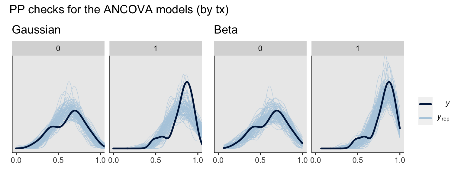
To my eye, a few broad patterns emerged. First, the ANCOVA versions of the model did better jobs simulating new data sets which better mimicked the distributions of the sample data. Second, the beta models did a better job capturing the skew in the data, particularly for the experimental group, than the Gaussian models. Along those lines, whereas the beta models respected the \((0, 1)\) bounds of the data, the Gaussian models did not, particularly for the experimental group.

Now we’ll do another version of a posterior-predictive check. This time we’ll plot the fitted lines for the two ANCOVA models across the full range of the baseline covariate pre.

# save a character vector to streamline the code below
likelihoods <- c("Gaussian", "beta")

# define the predictor grid
nd <- crossing(txf = factor(0:1),
               pre = seq(from = 0.001, to = 0.999, length.out = 400)) %>% 
  mutate(prec  = pre - mean(hoorelbeke2021$pre),
         prelo = qlogis(pre))


bind_rows(
  # compute the Gaussian fitted line
  fitted(fit2g, newdata = nd) %>% 
    data.frame() %>% 
    bind_cols(nd),
  # compute the beta fitted line
  fitted(fit2b, newdata = nd) %>% 
    data.frame() %>% 
    bind_cols(nd)
) %>% 
  # wrangle
  mutate(likelihood = rep(likelihoods, each = n() / 2) %>% factor(levels = likelihoods),
         tx         = ifelse(txf == "0", "control", "treatment")) %>% 
  
  # plot!
  ggplot(aes(x = pre)) +
  geom_hline(yintercept = 0:1, color = "white") +
  geom_vline(xintercept = 0:1, color = "white") +
  geom_ribbon(aes(ymin = Q2.5, ymax = Q97.5, fill = likelihood),
              linewidth = 0, alpha = 1/2) +
  geom_point(data = hoorelbeke2021 %>% 
               mutate(tx = ifelse(txf == "0", "control", "treatment")),
             aes(y = post)) +
  scale_fill_viridis_d(option = "H", begin = .2, end = .8) +
  scale_x_continuous(breaks = 0:5 / 5) +
  scale_y_continuous(breaks = 0:5 / 5) +
  coord_equal(xlim = 0:1,
              ylim = 0:1) +
  ggtitle("Fitted 95% CI ribbons for the ANCOVA's") +
  facet_wrap(~ tx)

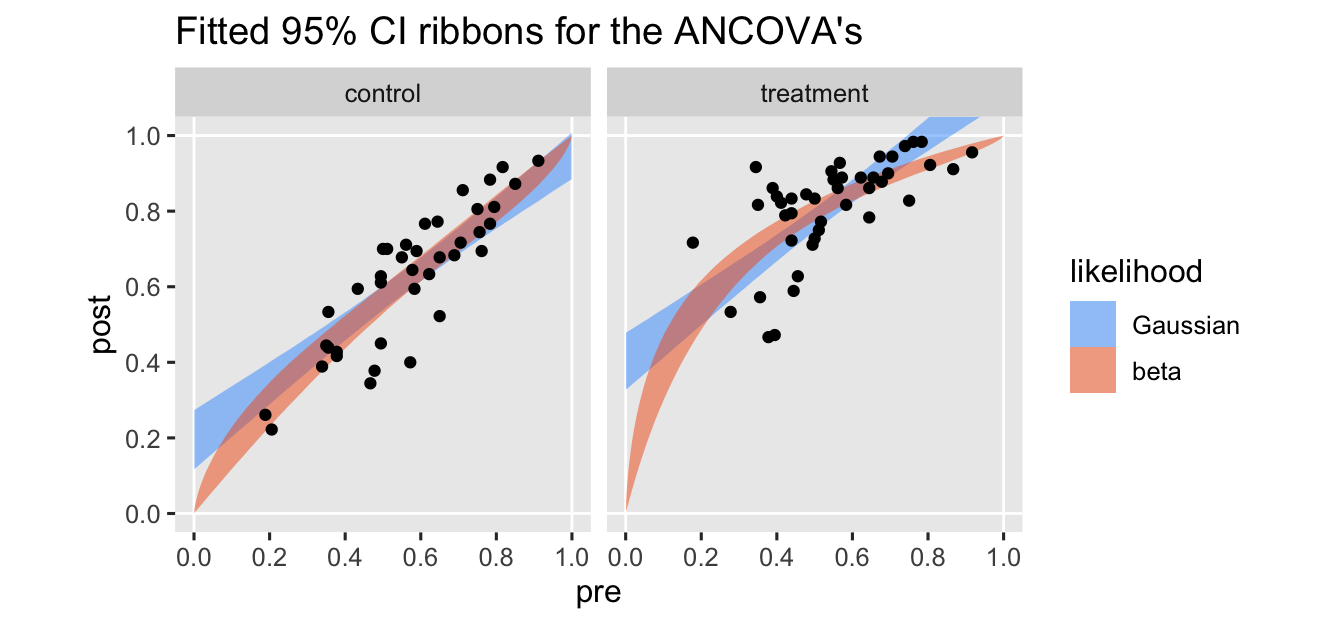
I’ve omitted the typical fitted lines for the posterior means from these plots to keep down the clutter. The vertical and horizontal white lines at the edges of the panels mark off the \((0, 1)\) boundaries for both axes. As expected, the predictions from the beta model respect the boundaries across the full range of the baseline covariate variable pre. The predictions for the Gaussian model, however, cross the upper limit at the higher values for pre, especially for those in the treatment condition.

Beta AN[C]OVA and potential outcomes

Posterior predicative checks are fun and interesting, but our main goal in this blog and this series has to do with causal inference, most often expressed in terms of the average treatment effect (ATE, \(\tau_\text{ATE}\)). In the subsections to follow, we’ll connect our beta-regression approach to the potential-outcomes framework. We start by discussing \(\beta\) coefficients.

Can the \(\beta\) coefficients help us estimate the ATE?

We already know that when you’re using simple Gaussian models, be they ANOVA’s or ANCOVA’s, the \(\beta_1\) parameter alone is a valid estimator of \(\tau_\text{ATE}\). Sadly, this will not be the case for beta-regression models using the logit link. Just like with logistic regression models for binary data, we can compute the ATE with a combination of both \(\beta_0\) and \(\beta_1\) for the beta ANOVA with the equation

$$\operatorname{logit}^{-1}(\beta_0 + \beta_1) - \operatorname{logit}^{-1}(\beta_1),$$

where \(\operatorname{logit}^{-1}(\cdot)\) is the inverse of the logit function (i.e., plogis()).⁷ Here’s how to work with the as_draws_df() output for fit1b to plot the full posterior distribution for the ATE. For kicks, we’ll even compare our ATE posterior with the sample ATE (SATE), as computed by hand with sample statistics.

# posttreatment mean for control
m_y0 <- hoorelbeke2021 %>% 
  filter(tx == 0) %>% 
  summarise(m_y0 = mean(post)) %>% 
  pull()

# posttreatment mean for treatment
m_y1 <- hoorelbeke2021 %>% 
  filter(tx == 1) %>% 
  summarise(m_y1 = mean(post)) %>% 
  pull()

# wrangle the posterior draws
as_draws_df(fit1b) %>% 
  mutate(ate = plogis(b_Intercept + b_txf1) - plogis(b_Intercept)) %>% 
  
  # plot
  ggplot(aes(x = ate)) +
  stat_halfeye(.width = c(.5, .95)) +
  # add in the SATE
  geom_vline(xintercept = m_y1 - m_y0, linetype = 2) +
  scale_y_continuous(NULL, breaks = NULL) +
  labs(title = "Our causal estimand from the Bayesian beta ANOVA",
       subtitle = "The dashed line marks the sample average treatment effect (SATE).",
       x = expression(hat(tau)[ATE]))

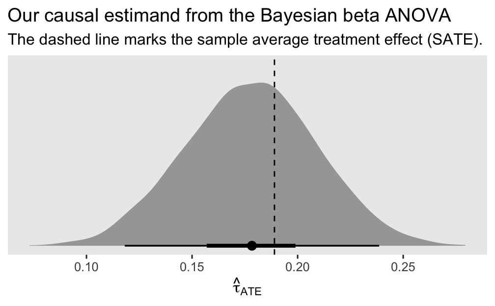
Since we used an MCMC-based Bayesian model with regularizing priors, we should not expect the posterior for \(\tau_\text{ATE}\) to center perfectly on top of the SATE. But it came pretty close and the SATE is comfortably captured within the inner 50% range of the posterior. I’d say this is a success.

Sadly, I am not aware of any way to use the \(\beta_1\) coefficient alone, nor any simple combination of all of the \(\beta\) coefficients, to hand compute the ATE with a beta-regression ANCOVA model. Much like with logistic regression for binary data, we must rely on the standardization approach, which we’ll rehearse in a moment. In the meantime, let’s compare the \(\beta_1\) estimates for the beta ANOVA and ANCOVA models.

rbind(fixef(fit1b)["txf1", ], fixef(fit2b)["txf1", ]) %>% 
  data.frame() %>% 
  mutate(fit = c("fit1b", "fit2b"),
         model_type = c("beta ANOVA", "beta ANCOVA")) %>%
  rename(`beta[1]` = Estimate) %>% 
  select(fit, model_type, `beta[1]`, Est.Error)

##     fit  model_type   beta[1] Est.Error
## 1 fit1b  beta ANOVA 0.9019085 0.1586365
## 2 fit2b beta ANCOVA 1.1326806 0.1138906

If you recall back to the third post in this series, logistic regression models have the surprising characteristic that the standard error (or posterior standard deviation) for the \(\beta_1\) coefficient usually increases when we add the baseline covariates to the model ( Ford & Norrie, 2002; Robinson & Jewell, 1991). Interestingly enough, that was not the case for our beta-regression models with the logit link. Rather, the posterior SD decreased in the beta ANCOVA, much like we’d expect from a Gaussian model. Frankly, I don’t have enough experience with beta models to know if this is a fluke with this sample, or if it’s a more general pattern, and I am not aware of any theoretical/methodological work that hashes out the details of how one might combine the potential-outcomes framework with beta regression. So for now, friends, we just get to sit with one another wrapped in our curiosity.

Beta ANOVA and the ATE.

As we’ve rehearsed in many earlier posts, we can compute our primary causal estimand \(\tau_\text{ATE}\) in two ways with an ANOVA model:

$$\tau_\text{ATE} = \mathbb E (y_i^1 - y_i^0) = \mathbb E (y_i^1) - \mathbb E (y_i^0).$$

For count and binary data, the group means are on different scales as the underlying data, which makes for some conceptual complications. But as we’ve seen with Gaussian and gamma data, the group means from a beta model are on the same scale as the underlying data; all the values range between 0 and 1, which will make our computations relatively easy, at least conceptually.

Beta ANOVA and \(\mathbb E (y_i^1) - \mathbb E (y_i^0)\).

As we’ve done in other posts showcasing Bayesian models, let’s streamline some of our summarizing code with a custom function. Many of the functions from the brms package summarize the posterior draws in terms of their mean, standard deviation, and percentile-based 95% intervals. Here we’ll make a custom function that will compute those summary statistics for all vectors in a data frame.

brms_summary <- function(x) {
  posterior::summarise_draws(x, "mean", "sd",  ~quantile(.x, probs = c(0.025, 0.975)))
}

Here’s how we might compute \(\hat{\tau}_\text{ATE}\) with the \(\mathbb E (y_i^1) - \mathbb E (y_i^0)\) approach via a fitted()-based workflow and our nice brms_summary() function.

# define the predictor grid
nd <- tibble(txf = 0:1)

# compute
fitted(fit1b,
       newdata = nd,
       summary = F) %>% 
  # wrangle
  data.frame() %>% 
  set_names(pull(nd, txf)) %>% 
  mutate(ate = `1` - `0`) %>% 
  # summarize!
  brms_summary()

## # A tibble: 3 × 5
##   variable  mean     sd `2.5%` `97.5%`
##   <chr>    <num>  <num>  <num>   <num>
## 1 0        0.627 0.0257  0.576   0.676
## 2 1        0.805 0.0190  0.766   0.841
## 3 ate      0.178 0.0310  0.118   0.239

The first two rows of the output are the posterior summaries for \(\mathbb E (y_i^0)\) and \(\mathbb E (y_i^1)\), and the final row is the summary for our focal estimate \(\hat{\tau}_\text{ATE}\).

Here’s the thrifty alternative martinaleffects-based workflow.

# change the default summary from the median to the mean
options(marginaleffects_posterior_center = mean)

# compute the predicted means
predictions(fit1b, newdata = nd, by = "txf")

## 
##  txf Estimate 2.5 % 97.5 %
##    0    0.627 0.576  0.676
##    1    0.805 0.766  0.841
## 
## Columns: rowid, txf, estimate, conf.low, conf.high, post

# compute the ATE
predictions(fit1b, newdata = nd, by = "txf", hypothesis = "revpairwise")

## 
##   Term Estimate 2.5 % 97.5 %
##  1 - 0    0.178 0.118  0.239
## 
## Columns: term, estimate, conf.low, conf.high

You’ll note that by default, both fitted() and predictions() returned the results in the \((0, 1)\) metric, rather than the log-odds scale of the model. When you’re working with non-identity link functions, pay close attention to the default settings for your functions, friends. They’ll get you.

Beta ANOVA and \(\mathbb E (y_i^1 - y_i^0)\).

As we’ve seen in other posts, before we compute our Bayesian posterior estimate for the ATE with the \(\mathbb E (y_i^1 - y_i^0)\) method, we’ll first need to redefine our nd predictor grid to contain both values of our grouping variable txf for each level of id.

nd <- hoorelbeke2021 %>% 
  select(id) %>% 
  expand_grid(txf = 0:1) %>% 
  mutate(row = 1:n())

# what?
glimpse(nd)

## Rows: 164
## Columns: 3
## $ id  <dbl> 1, 1, 2, 2, 3, 3, 4, 4, 5, 5, 6, 6, 7, 7, 8, 8, 9, 9, 10, 10, 11, 11, 12, 12, 13, 13, 14, 14, 16…
## $ txf <int> 0, 1, 0, 1, 0, 1, 0, 1, 0, 1, 0, 1, 0, 1, 0, 1, 0, 1, 0, 1, 0, 1, 0, 1, 0, 1, 0, 1, 0, 1, 0, 1, …
## $ row <int> 1, 2, 3, 4, 5, 6, 7, 8, 9, 10, 11, 12, 13, 14, 15, 16, 17, 18, 19, 20, 21, 22, 23, 24, 25, 26, 2…

We added that row index to help us join our nd predictor data to the fitted() output, below. Here’s the long block of fitted()-based code, annotated to help clarify the steps.

# compute the posterior predictions
fitted(fit1b,
       newdata = nd,
       summary = F) %>% 
  # convert the results to a data frame
  data.frame() %>% 
  # rename the columns
  set_names(pull(nd, row)) %>% 
  # add a numeric index for the MCMC draws
  mutate(draw = 1:n()) %>% 
  # convert to the long format
  pivot_longer(-draw) %>% 
  # convert the row column from the character format to the numeric format
  mutate(row = as.double(name)) %>% 
  # join the nd predictor grid to the output
  left_join(nd, by = "row") %>% 
  # drop two of the columns which are now unnecessary
  select(-name, -row) %>% 
  # convert to a wider format so we can compute the contrast
  pivot_wider(names_from = txf, values_from = value) %>% 
  # compute the ATE contrast
  mutate(tau = `1` - `0`) %>% 
  # compute the average ATE value within each MCMC draw
  group_by(draw) %>% 
  summarise(ate = mean(tau)) %>% 
  # remove the draw index column
  select(ate) %>% 
  # now summarize the ATE across the MCMC draws
  brms_summary()

## # A tibble: 1 × 5
##   variable  mean     sd `2.5%` `97.5%`
##   <chr>    <num>  <num>  <num>   <num>
## 1 ate      0.178 0.0310  0.118   0.239

We can also make the same computation with the marginaleffects::avg_comparisons() function, but with much thriftier code.

avg_comparisons(fit1b, variables = "txf")

## 
##  Term Contrast Estimate 2.5 % 97.5 %
##   txf    1 - 0    0.178 0.118  0.239
## 
## Columns: term, contrast, estimate, conf.low, conf.high

Sadly, that version of the output does not include the value for the posterior SD. If you really wanted that SD, though, you can use this little trick with help from the posterior_draws() function.

avg_comparisons(fit1b, variables = "txf") %>% 
  posterior_draws() %>% 
  select(draw) %>%
  brms_summary()

## # A tibble: 1 × 5
##   variable  mean     sd `2.5%` `97.5%`
##   <chr>    <num>  <num>  <num>   <num>
## 1 draw     0.178 0.0310  0.118   0.239

Boom!

Beta ANCOVA and the ATE.

To expand our theoretical framework to ANCOVA-type models, let \(\mathbf C_i\) stand a vector of continuous covariates and let \(\mathbf D_i\) stand a vector of discrete covariates, both of which vary across the \(i\) cases. We can use these to help estimate the ATE from the beta ANCOVA with the formula

$$\tau_\text{ATE} = \mathbb E (y_i^1 - y_i^0 \mid \mathbf C_i, \mathbf D_i),$$

where \(y_i^1\) and \(y_i^0\) are the counterfactual outcomes for each of the \(i\) cases, estimated in light of their covariate values. This is often called standardization or g-computation, but this time applied to beta models.

As we have seen in may other contexts where our models used a non-identity link, I am not aware of any way to compute the ATE from a beta ANCOVA with the group mean difference approach. That is,

$$ \tau_\text{CATE} = \operatorname{\mathbb{E}} (y_i^1 \mid \mathbf C = \mathbf c, \mathbf D = \mathbf d) - \operatorname{\mathbb{E}}(y_i^0 \mid \mathbf C = \mathbf c, \mathbf D = \mathbf d), $$

where the resulting estimand is the conditional ATE (i.e., CATE). In that equation, \(\mathbf C = \mathbf c\) is meant to convey you have chosen particular values \(\mathbf c\) for the variables in the \(\mathbf C\) vector, and \(\mathbf D = \mathbf d\) is meant to convey you have chosen particular values \(\mathbf d\) for the variables in the \(\mathbf D\) vector. In addition to central tendencies like means or modes, these values could be any which are of particular interest to researchers and their audiences. But the main point here is that in the case of the beta ANCOVA with the logit link,

$$ \tau_\text{ATE} \neq \tau_\text{CATE}. $$

If we want to improve our estimates of the ATE with baseline covariates, we need to use the standardization approach.

Beta ANCOVA and \(\mathbb E (y_i^1 - y_i^0 \mid \mathbf C_i, \mathbf D_i)\).

Before we compute our \(\hat \tau_\text{ATE}\) from the beta ANCOVA, we’ll want to expand our nd predictor grid to include the values for the pre covariate and its transformations.

nd <- hoorelbeke2021 %>% 
  select(id, pre, prec, prelo) %>% 
  expand_grid(txf = 0:1) %>% 
  mutate(row = 1:n())

# what?
glimpse(nd)

## Rows: 164
## Columns: 6
## $ id    <dbl> 1, 1, 2, 2, 3, 3, 4, 4, 5, 5, 6, 6, 7, 7, 8, 8, 9, 9, 10, 10, 11, 11, 12, 12, 13, 13, 14, 14, …
## $ pre   <dbl> 0.3444444, 0.3444444, 0.5111111, 0.5111111, 0.5833333, 0.5833333, 0.6444444, 0.6444444, 0.6944…
## $ prec  <dbl> -0.213821139, -0.213821139, -0.047154472, -0.047154472, 0.025067750, 0.025067750, 0.086178861,…
## $ prelo <dbl> -0.64355024, -0.64355024, 0.04445176, 0.04445176, 0.33647224, 0.33647224, 0.59470711, 0.594707…
## $ txf   <int> 0, 1, 0, 1, 0, 1, 0, 1, 0, 1, 0, 1, 0, 1, 0, 1, 0, 1, 0, 1, 0, 1, 0, 1, 0, 1, 0, 1, 0, 1, 0, 1…
## $ row   <int> 1, 2, 3, 4, 5, 6, 7, 8, 9, 10, 11, 12, 13, 14, 15, 16, 17, 18, 19, 20, 21, 22, 23, 24, 25, 26,…

Still building up to the main event, let’s make a couple plots. Here we compute and then display the \(\hat y_i^1\) and \(\hat y_i^0\) values for each participant. For comparison sake, we’ll include the estimates for both Gaussian and beta ANCOVA’s.

# save a character vector to streamline the code below
likelihoods <- c("Gaussian", "beta")

# compute the counterfactual predictions for each case
bind_rows(
  predictions(fit2g, newdata = nd, by = c("id", "txf", "pre")),
  predictions(fit2b, newdata = nd, by = c("id", "txf", "pre"))
) %>% 
  # wrangle
  data.frame() %>% 
  mutate(y = ifelse(txf == 0, "hat(italic(y))^0", "hat(italic(y))^1")) %>% 
  mutate(likelihood = rep(likelihoods, each = n() / 2) %>% factor(levels = likelihoods)) %>% 
  
  # plot!
  ggplot(aes(x = estimate, y = reorder(id, estimate))) +
  geom_vline(xintercept = 0:1, color = "white") +
  geom_interval(aes(xmin = conf.low, xmax = conf.high, color = y),
                    position = position_dodge(width = -0.2),
                    size = 1/5) +
  geom_point(aes(color = y, shape = y),
             size = 2) +
  scale_color_viridis_d(NULL, option = "A", begin = .3, end = .6,
                        labels = scales::parse_format()) +
  scale_shape_manual(NULL, values = c(20, 18),
              labels = scales::parse_format()) +
  scale_x_continuous(breaks = 0:5 / 5) +
  scale_y_discrete(breaks = NULL) +
  labs(title = "Counterfactual predictions",
       x = "post",
       y = "id (ranked)") +
  coord_cartesian(xlim = 0:1) +
  theme(legend.background = element_blank(),
        legend.position = c(.58, .85)) +
  facet_wrap(~ likelihood, labeller = label_both)

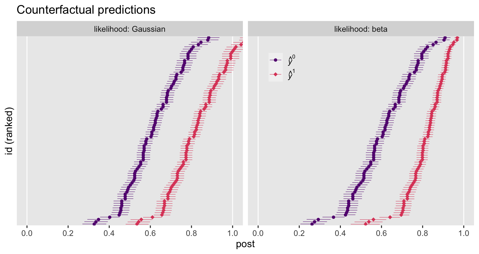
The counterfactual estimates between the Gaussian and beta ANCOVA’s do share a similar gross structure. But notice how the Gaussian-based estimates happily blow right past the right-hand boundary of 1, whereas the beta-based estimates restrict themselves within the range in which they belong. Now let’s compute and plot the contrasts.

bind_rows(
  comparisons(fit2g, variables = "txf", by = "id"),
  comparisons(fit2b, variables = "txf", by = "id")
) %>% 
  data.frame() %>% 
  mutate(likelihood = rep(likelihoods, each = n() / 2) %>% factor(levels = likelihoods)) %>% 
  
  ggplot(aes(x = estimate, y = reorder(id, estimate))) +
  geom_vline(xintercept = 0, color = "white") +
  geom_interval(aes(xmin = conf.low, xmax = conf.high),
                size = 1/5) +
  geom_point() +
  scale_y_discrete(breaks = NULL) +
  labs(title = "Treatment effects",
       x = expression(hat(tau)[italic(i)]~("i.e., "*hat(italic(y))[italic(i)]^1-hat(italic(y))[italic(i)]^0)),
       y = NULL) +
  xlim(-1, 1) +
  facet_grid(~ likelihood, labeller = label_both)

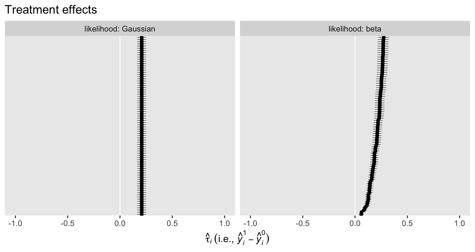
In this case, the logical boundaries for the contrasts are -1 and 1. I didn’t bother marking them off with vertical lines because the results from both models are well within their bounds. As has always been the case, the \(\hat \tau_i\) posteriors are all identical when computed from the Gaussian ANCOVA (using the identity link), but they do differ from one another when computed from our logit-link beta model, don’t they? This is why when we use a beta ANCOVA with a non-identity link, we must rely on the standardization method when computing the ATE. Speaking of which, here’s how to compute \(\hat{\tau}_\text{ATE}\) for our two ANCOVA’s with the nice avg_comparisons() function.

bind_rows(
  avg_comparisons(fit2g, variables = "txf"),
  avg_comparisons(fit2b, variables = "txf")
) %>% 
  data.frame() %>%
  mutate(likelihood = factor(likelihoods, levels = likelihoods),
         link       = c("identity", "logit")) %>% 
  select(likelihood, link, estimate, starts_with("conf")) %>%
  mutate_if(is.double, round, digits = 3)

##   likelihood     link estimate conf.low conf.high
## 1   Gaussian identity    0.208    0.164     0.249
## 2       beta    logit    0.207    0.166     0.246

In this case, the results between the two likelihoods are very similar. Though notice the 95% interval appears a little narrower with the beta model. Let’s augment our workflow with the posterior_draws() function so we can compute their posterior SD’s.

bind_rows(
  avg_comparisons(fit2g, variables = "txf") %>% posterior_draws(),
  avg_comparisons(fit2b, variables = "txf") %>% posterior_draws()
) %>% 
  rename(ate = draw) %>% 
  mutate(likelihood = rep(likelihoods, each = n() / 2) %>% factor(levels = likelihoods)) %>% 
  select(likelihood, ate) %>% 
  group_by(likelihood) %>% 
  brms_summary() %>%
  mutate_if(is.double, round, digits = 4)

## # A tibble: 2 × 6
## # Groups:   likelihood [2]
##   likelihood variable  mean     sd `2.5%` `97.5%`
##   <fct>      <chr>    <dbl>  <dbl>  <dbl>   <dbl>
## 1 Gaussian   ate      0.208 0.0219  0.164   0.249
## 2 beta       ate      0.207 0.0201  0.166   0.246

Yep, look at that. The beta ANCOVA gave us a more precise estimate of the ATE by the 95% interval width and the posterior SD. I’d want to see a simulation study or something before I made any broad claims about greater precision with the beta ANCOVA versus the Gaussian ANCOVA. Regardless of the magnitude of the posterior SD, I’d much rather use the beta ANCOVA for computing my \(\hat{\tau}_\text{ATE}\) because it’s just silly to presume \((0, 1)\) interval data will follow a Gaussian distribution. The beta likelihood is a much better conceptual fit, and I’d love to see my fellow scientists using the beta ANCOVA more frequently in their work.

We should investigate whether the beta ANCOVA did indeed return a more precise estimate for the ATE, relative to the beta ANOVA.

bind_rows(
  avg_comparisons(fit1b, variables = "txf") %>% posterior_draws(),
  avg_comparisons(fit2b, variables = "txf") %>% posterior_draws()
) %>% 
  rename(ate = draw) %>% 
  mutate(model = rep(c("beta ANOVA", "beta ANCOVA"), each = n() / 2) %>% factor(levels = c("beta ANOVA", "beta ANCOVA"))) %>% 
  select(model, ate) %>% 
  group_by(model) %>% 
  brms_summary() %>%
  mutate_if(is.double, round, digits = 3)

## # A tibble: 2 × 6
## # Groups:   model [2]
##   model       variable  mean    sd `2.5%` `97.5%`
##   <fct>       <chr>    <dbl> <dbl>  <dbl>   <dbl>
## 1 beta ANOVA  ate      0.178 0.031  0.118   0.239
## 2 beta ANCOVA ate      0.207 0.02   0.166   0.246

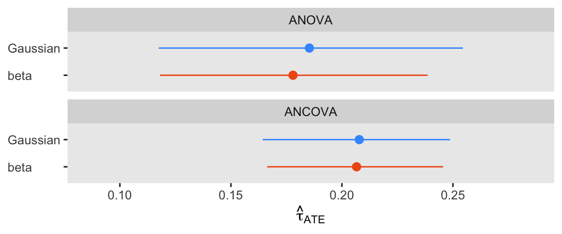
Yep, adding the pre score to the beta ANCOVA returned a smaller posterior SD and a narrower 95% interval. If you can add a high-quality baseline covariate or 2 to your beta model, you probably should. For kicks and giggles, let’s finish this section out with a coefficient plot of the \(\hat{\tau}_\text{ATE}\) from all 4 models.

bind_rows(
  avg_comparisons(fit1g, variables = "txf"),
  avg_comparisons(fit1b, variables = "txf"),
  avg_comparisons(fit2g, variables = "txf"),
  avg_comparisons(fit2b, variables = "txf")
) %>% 
  data.frame() %>%
  mutate(likelihood = rep(likelihoods, times = 2) %>% factor(levels = likelihoods),
         model      = rep(c("ANOVA", "ANCOVA"), each = 2) %>% factor(levels = c("ANOVA", "ANCOVA"))) %>% 
  
  ggplot(aes(x = estimate, xmin = conf.low, xmax = conf.high, y = fct_rev(likelihood))) +
  geom_pointrange(aes(color = likelihood),
                  show.legend = F) +
  scale_x_continuous(expression(hat(tau)[ATE]), expand = expansion(mult = 0.3)) +
  scale_color_viridis_d(option = "H", begin = .2, end = .8, direction = 1) +
  ylab(NULL) +
  facet_wrap(~ model, nrow = 2) +
  theme(axis.text.y = element_text(hjust = 0))

What about 0 and 1?

So far in this post, we’ve largely described the pre and post variables in the hoorelbeke2021 data as if they’re bound within the \((0, 1)\) interval. I’m no aPASAT expert, but I suspect those aPASAT scores can technically take on values of 0 and 1, too. Even if I’m wrong in this special case, sometimes researchers have \([0, 1]\) data, and in those cases the simple beta likelihood just won’t work. Happily for us, our friends the statisticians and methodologists have already proposed zero-or-one-inflated beta models ( Ospina & Ferrari, 2012), zero-and-one inflated beta models ( Swearingen et al., 2012), and ordered beta models ( Kubinec, 2022). Zero-, one-, and zero-and-one inflated beta models are natively available with brms ( Bürkner, 2023c). To my knowledge, ordered beta models are only indirectly available with brms through the ordbetareg package ( Kubinec, 2023), at the moment.

How about intervals other than 0 and 1?

Sometimes interval-bounded continuous data have an upper limit other than 1, and/or a lower limit other than 0. The current go-to solution with brms and other packages is to just rescale your data to the \((0, 1)\) or \([0, 1]\) range prior to the analysis, and then fit a variant of a beta model with our without inflation. However, there is such a thing as a four-parameter beta distribution which includes a shift parameter to adjust the lower limit and a scale parameter to adjust the upper limit. See here for a quick reference. To my knowledge, the only way to actually fit such a model without rescaling the data involves making a custom likelihood in brms, which you can learn about in Bürkner’s ( 2023b) vignette, Define custom response distributions with brms.

Recap

In this post, some of the main points we covered were:

• The beta likelihood is designed for continuous data bounded between 0 and 1. It is not conventionally included within the GLM family, but may be thought of as falling within a broader class of models with arbitrary likelihood functions.
• I’m not aware there is a canonical link for beta models, but I recommend the logit link, which is the default for brms.
• For the beta ANOVA, the \(\mathbb E (y_i^1 - y_i^0)\) method and the \(\mathbb E (y_i^1) - \mathbb E (y_i^0)\) method are both valid estimators of \(\tau_\text{ATE}\).
• For the beta ANCOVA, the only valid estimator of \(\tau_\text{ATE}\) is the \(\mathbb E (y_i^1 - y_i^0)\) method, which we typically refer to as standardization in this blog series.
• Finally, it does appear that the beta ANCOVA will return more precise estimates of the ATE than the simple beta ANOVA. Use your baseline covariates!

In the next post, we’ll shift gears and introduce the analysis of heterogeneous covariance (ANHECOVA) for causal inference.

Session info

sessionInfo()

## R version 4.3.0 (2023-04-21)
## Platform: aarch64-apple-darwin20 (64-bit)
## Running under: macOS Ventura 13.4
## 
## Matrix products: default
## BLAS:   /Library/Frameworks/R.framework/Versions/4.3-arm64/Resources/lib/libRblas.0.dylib 
## LAPACK: /Library/Frameworks/R.framework/Versions/4.3-arm64/Resources/lib/libRlapack.dylib;  LAPACK version 3.11.0
## 
## locale:
## [1] en_US.UTF-8/en_US.UTF-8/en_US.UTF-8/C/en_US.UTF-8/en_US.UTF-8
## 
## time zone: America/Chicago
## tzcode source: internal
## 
## attached base packages:
## [1] stats     graphics  grDevices utils     datasets  methods   base     
## 
## other attached packages:
##  [1] marginaleffects_0.12.0 tidybayes_3.0.4        patchwork_1.1.2        brms_2.19.0           
##  [5] Rcpp_1.0.10            lubridate_1.9.2        forcats_1.0.0          stringr_1.5.0         
##  [9] dplyr_1.1.2            purrr_1.0.1            readr_2.1.4            tidyr_1.3.0           
## [13] tibble_3.2.1           ggplot2_3.4.2          tidyverse_2.0.0       
## 
## loaded via a namespace (and not attached):
##   [1] tensorA_0.36.2       rstudioapi_0.14      jsonlite_1.8.5       magrittr_2.0.3       TH.data_1.1-2       
##   [6] estimability_1.4.1   farver_2.1.1         nloptr_2.0.3         rmarkdown_2.22       vctrs_0.6.3         
##  [11] minqa_1.2.5          base64enc_0.1-3      blogdown_1.17        htmltools_0.5.5      haven_2.5.2         
##  [16] distributional_0.3.2 sass_0.4.6           StanHeaders_2.26.27  bslib_0.5.0          htmlwidgets_1.6.2   
##  [21] plyr_1.8.8           sandwich_3.0-2       emmeans_1.8.6        zoo_1.8-12           cachem_1.0.8        
##  [26] igraph_1.4.3         mime_0.12            lifecycle_1.0.3      pkgconfig_2.0.3      colourpicker_1.2.0  
##  [31] Matrix_1.5-4         R6_2.5.1             fastmap_1.1.1        collapse_1.9.6       shiny_1.7.4         
##  [36] digest_0.6.31        colorspace_2.1-0     ps_1.7.5             crosstalk_1.2.0      projpred_2.6.0      
##  [41] labeling_0.4.2       fansi_1.0.4          timechange_0.2.0     abind_1.4-5          mgcv_1.8-42         
##  [46] compiler_4.3.0       withr_2.5.0          backports_1.4.1      inline_0.3.19        shinystan_2.6.0     
##  [51] gamm4_0.2-6          highr_0.10           pkgbuild_1.4.1       MASS_7.3-58.4        gtools_3.9.4        
##  [56] loo_2.6.0            tools_4.3.0          httpuv_1.6.11        threejs_0.3.3        glue_1.6.2          
##  [61] callr_3.7.3          nlme_3.1-162         promises_1.2.0.1     grid_4.3.0           checkmate_2.2.0     
##  [66] reshape2_1.4.4       generics_0.1.3       gtable_0.3.3         tzdb_0.4.0           data.table_1.14.8   
##  [71] hms_1.1.3            utf8_1.2.3           pillar_1.9.0         ggdist_3.3.0         markdown_1.7        
##  [76] posterior_1.4.1      later_1.3.1          splines_4.3.0        lattice_0.21-8       survival_3.5-5      
##  [81] tidyselect_1.2.0     miniUI_0.1.1.1       knitr_1.43           arrayhelpers_1.1-0   gridExtra_2.3       
##  [86] bookdown_0.34        stats4_4.3.0         xfun_0.39            bridgesampling_1.1-2 matrixStats_1.0.0   
##  [91] DT_0.28              rstan_2.21.8         stringi_1.7.12       yaml_2.3.7           boot_1.3-28.1       
##  [96] evaluate_0.21        codetools_0.2-19     emo_0.0.0.9000       cli_3.6.1            RcppParallel_5.1.7  
## [101] shinythemes_1.2.0    xtable_1.8-4         munsell_0.5.0        processx_3.8.1       jquerylib_0.1.4     
## [106] coda_0.19-4          svUnit_1.0.6         parallel_4.3.0       rstantools_2.3.1     ellipsis_0.3.2      
## [111] assertthat_0.2.1     prettyunits_1.1.1    dygraphs_1.1.1.6     bayesplot_1.10.0     Brobdingnag_1.2-9   
## [116] lme4_1.1-33          viridisLite_0.4.2    mvtnorm_1.2-2        scales_1.2.1         xts_0.13.1          
## [121] insight_0.19.2       crayon_1.5.2         rlang_1.1.1          multcomp_1.4-24      shinyjs_2.1.0

References

Brooks, M. E., Kristensen, K., van Benthem, K. J., Magnusson, A., Berg, C. W., Nielsen, A., Skaug, H. J., Maechler, M., & Bolker, B. M. (2017). glmmTMB balances speed and flexibility among packages for zero-inflated generalized linear mixed modeling. The R Journal, 9(2), 378–400. https://doi.org/10.32614/RJ-2017-066
Brooks, M., Bolker, B., Kristensen, K., Maechler, M., Magnusson, A., Skaug, H., Nielsen, A., Berg, C., & van Bentham, K. (2023). glmmTMB: Generalized linear mixed models using template model builder [Manual]. https://github.com/glmmTMB/glmmTMB
Bürkner, P.-C. (2023a). brms reference manual, Version 2.19.0. https://CRAN.R-project.org/package=brms/brms.pdf
Bürkner, P.-C. (2023b). Define custom response distributions with brms. https://CRAN.R-project.org/package=brms/vignettes/brms_customfamilies.html
Bürkner, P.-C. (2023c). Parameterization of response distributions in brms. https://CRAN.R-project.org/package=brms/vignettes/brms_families.html
Cribari-Neto, F., & Zeileis, A. (2010). Beta regression in R. Journal of Statistical Software, 34(2), 1–24. https://doi.org/10.18637/jss.v034.i02
Ferrari, S., & Cribari-Neto, F. (2004). Beta regression for modelling rates and proportions. Journal of Applied Statistics, 31(7), 799–815. https://doi.org/10.1080/0266476042000214501
Ford, I., & Norrie, J. (2002). The role of covariates in estimating treatment effects and risk in long-term clinical trials. Statistics in Medicine, 21(19), 2899–2908. https://doi.org/10.1002/sim.1294
Grün, B., Kosmidis, I., & Zeileis, A. (2012). Extended beta regression in R: Shaken, stirred, mixed, and partitioned. Journal of Statistical Software, 48(11), 1–25. https://doi.org/10.18637/jss.v048.i11
Hoorelbeke, K., Van den Bergh, N., De Raedt, R., Wichers, M., & Koster, E. H. (2021). Preventing recurrence of depression: Long-term effects of a randomized controlled trial on cognitive control training for remitted depressed patients. Clinical Psychological Science, 9(4), 615–633. https://doi.org/10.1177/21677026209797
Kubinec, R. (2022). Ordered beta regression: A parsimonious, well-fitting model for continuous data with lower and upper bounds. Political Analysis, 1–18. https://doi.org/10.1017/pan.2022.20
Kubinec, R. (2023). ordbetareg: Ordered beta regression models with brms [Manual]. https://CRAN.R-project.org/package=ordbetareg
Kurz, A. S. (2023a). Statistical Rethinking with brms, ggplot2, and the tidyverse (version 1.3.0). https://bookdown.org/content/3890/
Kurz, A. S. (2023b). Statistical Rethinking with brms, ggplot2, and the tidyverse: Second Edition (version 0.4.0). https://bookdown.org/content/4857/
McElreath, R. (2020). Statistical rethinking: A Bayesian course with examples in R and Stan (Second Edition). CRC Press. https://xcelab.net/rm/statistical-rethinking/
Nelder, J. A., & Wedderburn, R. W. (1972). Generalized linear models. Journal of the Royal Statistical Society: Series A (General), 135(3), 370–384. https://doi.org/10.2307/2344614
Ospina, R., & Ferrari, S. L. (2012). A general class of zero-or-one inflated beta regression models. Computational Statistics & Data Analysis, 56(6), 1609–1623. https://doi.org/10.1016/j.csda.2011.10.005
Paolino, P. (2001). Maximum likelihood estimation of models with beta-distributed dependent variables. Political Analysis, 9(4), 325–346. https://doi.org/10.1093/oxfordjournals.pan.a004873
Popoviciu, T. (1935). Sur les équations algébriques ayant toutes leurs racines réelles. Mathematica Cluj, 9(129-145).
Robinson, L. D., & Jewell, N. P. (1991). Some surprising results about covariate adjustment in logistic regression models. International Statistical Review/Revue Internationale de Statistique, 227–240. https://doi.org/10.2307/1403444
Swearingen, C. J., Castro, M. M., & Bursac, Z. (2012). Inflated beta regression: Zero, one, and everything in between. SAS Global Forum, 11.
Zeileis, A., Cribari-Neto, F., Gruen, B., & Kosmidis, I. (2021). betareg: Beta regression [Manual]. https://CRAN.R-project.org/package=betareg
-
If you didn’t know, when you have left- and right-bounded data, the sample distribution with the largest possible standard deviation is when half of the values are piled up on the lowest value, and the other half are piled up on the highest value. Try it out for yourself and see. You could also, of course, prove this with Popoviciu’s inequality ( Popoviciu, 1935), as I outlined in this blog post from a while back. ↩︎
If you’re a brms user not used to the
0 + Interceptsyntax, it’s hard to understate how important it is to learn. You can start by reading through my discussions here or here ( Kurz, 2023a, 2023b). Then study theset_priorandbrmsformulasections of the brms reference manual ( Bürkner, 2023a). In short, if you have not mean-centered all of your predictor variables, you might should use the0 + Interceptsyntax. In all 4 models in this blog post, thetxffactor variable is not mean centered, so0 + Interceptsyntax is the way to go. ↩︎ -
Even the binomial is only technically included as part of the exponential family when the number of trials
\(n\)is fixed. To my eye, it’s extremely uncommon to see a binomial model with a random\(n\), but it is possible, and I have even fit such a model withbrms::brm(). I only bring this up to show how restrictive and picky the exponential-family criterion can get. ↩︎ -
I am not an expert on this topic, but my current understanding is the beta distribution does not count as exponential when both
\(\alpha\)and\(\beta\)parameters are random. However, it can be considered as exponential when one or the other of those parameters are fixed. Sadly, I don’t have a nice reader-friendly source for this. Rather, it’s just something I picked up from searching around online. If you, dear reader, have a nice reader-friendly source that can be understood by non-PhD statisticians, I’d love to see it. In the meantime, here’s a Cross Validated thread on the topic. ↩︎ -
Go here for a completely non-authoritative poll on the topic. ↩︎
By now you may be asking yourself: But could I also use a gamma prior for
\(\sigma\)in the Gaussian models? Why yes, yes you could. If you wanted to be super extra, you could even use a gamma prior for\(\sigma\)that’s been truncated on the right at the upper limit of 0.5. Wouldn’t that be fun to slip into a paper? ↩︎ -
The inverse of the logit function, recall, is defined as
\(\operatorname{logit}^{-1}(p) = \exp(p)/[1 + \exp(p)]\). ↩︎
- Posted on:
- June 25, 2023
- Length:
- 43 minute read, 9074 words