Causal inference with gamma regression or: The problem is with the link function, not the likelihood

So far the difficulties we have seen with covaraites, causal inference, and the GLM have all been restricted to discrete models (e.g., binomial, Poisson, negative binomial). In this sixth post of the series, we’ll see this issue can extend to models for continuous data, too. As it turns out, it may have less to do with the likelihood function, and more to do with the choice of link function. To highlight the point, we’ll compare Gaussian and gamma models, with both the identity and log links.

We need data

In post, we’ll be continuing on with our horan1971 data set from the first, second, and fourth posts. These data, recall, were transposed from the values displayed in Table 2 from Horan & Johnson ( 1971). I’ve saved them as an external .rda file on my GitHub, which you can access using the code below. If you don’t want to pull a file from my GitHub, you can just copy the code from the first post.

# packages
library(tidyverse)
library(broom)
library(marginaleffects)
library(ggdist)
library(brms)
library(moments)
library(patchwork)

# adjust the global theme
theme_set(theme_gray(base_size = 12) +
            theme(panel.grid = element_blank()))

# load the data from GitHub
load(url("https://github.com/ASKurz/blogdown/raw/main/content/blog/2023-04-12-boost-your-power-with-baseline-covariates/data/horan1971.rda?raw=true"))

# wrangle a bit
horan1971 <- horan1971 %>% 
  filter(treatment %in% c("delayed", "experimental")) %>% 
  mutate(prec = pre - mean(pre),
         experimental = ifelse(treatment == "experimental", 1, 0))

# what are these, again?
glimpse(horan1971)

## Rows: 41
## Columns: 8
## $ sl           <chr> "a", "b", "c", "d", "e", "f", "g", "h", "i", "j", "k", "l", "m", "n", "o", "p", "q", "r…
## $ sn           <int> 1, 2, 3, 4, 5, 6, 7, 8, 9, 10, 11, 12, 13, 14, 15, 16, 17, 18, 19, 20, 21, 22, 62, 63, …
## $ treatment    <fct> delayed, delayed, delayed, delayed, delayed, delayed, delayed, delayed, delayed, delaye…
## $ pre          <dbl> 149.50, 131.25, 146.50, 133.25, 131.00, 141.00, 145.75, 146.75, 172.50, 156.50, 153.00,…
## $ post         <dbl> 149.00, 130.00, 147.75, 139.00, 134.00, 145.25, 142.25, 147.00, 158.25, 155.25, 151.50,…
## $ prec         <dbl> -5.335366, -23.585366, -8.335366, -21.585366, -23.835366, -13.835366, -9.085366, -8.085…
## $ delayed      <dbl> 1, 1, 1, 1, 1, 1, 1, 1, 1, 1, 1, 1, 1, 1, 1, 1, 1, 1, 1, 1, 1, 1, 0, 0, 0, 0, 0, 0, 0, …
## $ experimental <dbl> 0, 0, 0, 0, 0, 0, 0, 0, 0, 0, 0, 0, 0, 0, 0, 0, 0, 0, 0, 0, 0, 0, 1, 1, 1, 1, 1, 1, 1, …

Model framework

To my eye, gamma regression is one of the more under-used frameworks within the broader GLM framework.¹ Recall the dependent variable in the horan1971 data, post, is post-intervention weights, measured in pounds. Whether in humans or other animals, body weights are positive continuous values, and their distributions can often show a right skew, particularly whey their means are close to zero. Even though researchers often model data of this kind with the Gaussian likelihood, the gamma distribution can be a great alternative that easily accounts for the lower zero limit and any right skew.² The inverse link is the canonical link function for gamma regression models ( Nelder & Wedderburn, 1972). To give you a sense, the inverse link works like so:

tibble(lbs = seq(from = 0.1, to = 10, by = 0.01)) %>% 
  mutate(`1 / lbs` = 1 / lbs) %>% 
  
  ggplot(aes(x = lbs, y = `1 / lbs`)) +
  geom_hline(yintercept = 1, color = "white") +
  geom_vline(xintercept = 1, color = "white") +
  geom_line() +
  scale_x_continuous(breaks = c(0, 1, 5, 10)) +
  scale_y_continuous(breaks = c(0, 1, 5, 10)) +
  labs(subtitle = "The identity and inverse links for lbs. ranging from 0.1 to 10")

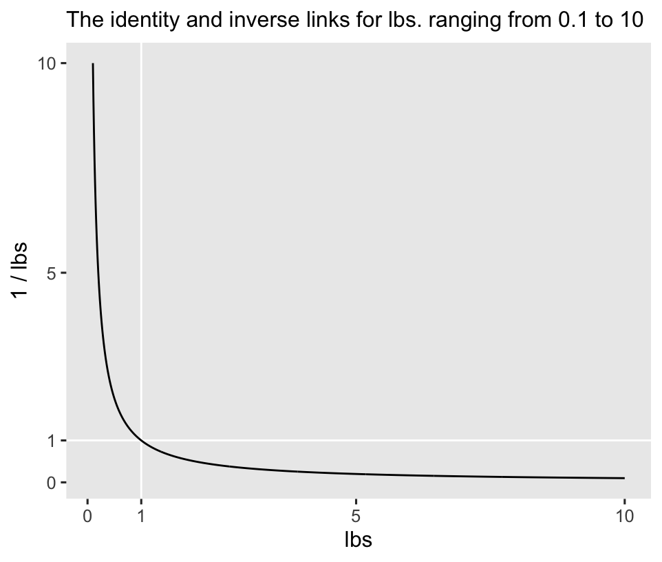
The inverse link has an elbow at 1, and it asymptotes at zero. However, I and others (e.g., Agresti, 2015; McCullagh & Nelder, 1989) have noticed the inverse link has its quirks³ for gamma regression, and the identity and log links make for good alternatives. In this blog post, we’ll explore gamma models with both identity and log links. Feel free to explore with the inverse link on your own. The overall results should be similar.

We will fit 8 models in total. To warm up, we will start by fitting 4 ANOVA models:

• Gaussian with the identity link,
• Gaussian with the log link,
• gamma with the identity link, and
• gamma with the log link.

Then we will get to the heart of the post by fitting 4 ANCOVA models:

• Gaussian with the identity link,
• Gaussian with the log link,
• gamma with the identity link, and
• gamma with the log link.

It’s easy with ANOVA.

If we start with the conventional Gaussian likelihood with the identity link as a benchmark, our first ANOVA-type model will follow the form

$$ \begin{align*} \text{post}_i & \sim \operatorname{Normal}(\mu_i, \sigma) \\ \mu_i & = \beta_0 + \beta_1 \text{experimental}_i, \end{align*} $$ where \(\beta_0\) is the mean for those on the control condition (i.e., delayed) and \(\beta_1\) is the difference in the mean for those in the treatment condition (i.e., experimental), relative to those in the control.

Our second model will use the log link, instead. Our third model will use the gamma likelihood, but retain the identity link. Our final ANOVA-type model will use the gamma likelihood and the log link. We’ll name the models glm1a through glm1d.

Here’s how to fit the models with maximum likelihood by way of the base-R glm() function. Take special note of the syntax we used in the family arguments.

# Gaussian, identity link
glm1a <- glm(
  data = horan1971,
  family = gaussian,
  post ~ 1 + experimental)

# Gaussian, log link
glm1b <- glm(
  data = horan1971,
  family = gaussian(link = "log"),
  post ~ 1 + experimental)

# gamma, identity link
glm1c <- glm(
  data = horan1971,
  family = Gamma(link = "identity"),
  post ~ 1 + experimental)

# gamma, log link
glm1d <- glm(
  data = horan1971,
  family = Gamma(link = "log"),
  post ~ 1 + experimental)

Review the parameter summaries.

summary(glm1a)

## 
## Call:
## glm(formula = post ~ 1 + experimental, family = gaussian, data = horan1971)
## 
## Coefficients:
##              Estimate Std. Error t value Pr(>|t|)    
## (Intercept)   153.818      3.674  41.864   <2e-16 ***
## experimental   -2.489      5.397  -0.461    0.647    
## ---
## Signif. codes:  0 '***' 0.001 '**' 0.01 '*' 0.05 '.' 0.1 ' ' 1
## 
## (Dispersion parameter for gaussian family taken to be 297.004)
## 
##     Null deviance: 11646  on 40  degrees of freedom
## Residual deviance: 11583  on 39  degrees of freedom
## AIC: 353.75
## 
## Number of Fisher Scoring iterations: 2

summary(glm1b)

## 
## Call:
## glm(formula = post ~ 1 + experimental, family = gaussian(link = "log"), 
##     data = horan1971)
## 
## Coefficients:
##              Estimate Std. Error t value Pr(>|t|)    
## (Intercept)   5.03577    0.02389 210.816   <2e-16 ***
## experimental -0.01632    0.03540  -0.461    0.647    
## ---
## Signif. codes:  0 '***' 0.001 '**' 0.01 '*' 0.05 '.' 0.1 ' ' 1
## 
## (Dispersion parameter for gaussian family taken to be 297.004)
## 
##     Null deviance: 11646  on 40  degrees of freedom
## Residual deviance: 11583  on 39  degrees of freedom
## AIC: 353.75
## 
## Number of Fisher Scoring iterations: 4

summary(glm1c)

## 
## Call:
## glm(formula = post ~ 1 + experimental, family = Gamma(link = "identity"), 
##     data = horan1971)
## 
## Coefficients:
##              Estimate Std. Error t value Pr(>|t|)    
## (Intercept)   153.818      3.706  41.508   <2e-16 ***
## experimental   -2.489      5.397  -0.461    0.647    
## ---
## Signif. codes:  0 '***' 0.001 '**' 0.01 '*' 0.05 '.' 0.1 ' ' 1
## 
## (Dispersion parameter for Gamma family taken to be 0.01276889)
## 
##     Null deviance: 0.49198  on 40  degrees of freedom
## Residual deviance: 0.48926  on 39  degrees of freedom
## AIC: 352.69
## 
## Number of Fisher Scoring iterations: 3

summary(glm1d)

## 
## Call:
## glm(formula = post ~ 1 + experimental, family = Gamma(link = "log"), 
##     data = horan1971)
## 
## Coefficients:
##              Estimate Std. Error t value Pr(>|t|)    
## (Intercept)   5.03577    0.02409 209.026   <2e-16 ***
## experimental -0.01632    0.03539  -0.461    0.647    
## ---
## Signif. codes:  0 '***' 0.001 '**' 0.01 '*' 0.05 '.' 0.1 ' ' 1
## 
## (Dispersion parameter for Gamma family taken to be 0.01276889)
## 
##     Null deviance: 0.49198  on 40  degrees of freedom
## Residual deviance: 0.48926  on 39  degrees of freedom
## AIC: 352.69
## 
## Number of Fisher Scoring iterations: 4

With both Gaussian and gamma likelihoods, the \(\beta_1\) parameter is the same as the estimate for \(\tau_\text{ATE}\) when we use the identity link. When we use the log link, however, we can compute the point estimate for \(\tau_\text{ATE}\) with the formula

$$\hat{\tau}_\text{ATE} = \exp(\hat \beta_0 + \hat \beta_1) - \exp(\hat \beta_0).$$

Here’s how to compute the \(\hat{\tau}_\text{ATE}\) values all by hand with the coef() function.

likelihoods <- c("Gaussian", "Gamma")
links <- c("identity", "log")

tibble(likelihood = rep(likelihoods, each = 2),
       link       = rep(links, times = 2),
       ate        = c(
         as.double(coef(glm1a)[2]),
         as.double(exp(coef(glm1b)[1] + coef(glm1b)[2]) - exp(coef(glm1b)[1])),
         as.double(coef(glm1c)[2]),
         as.double(exp(coef(glm1d)[1] + coef(glm1d)[2]) - exp(coef(glm1d)[1])))
)

## # A tibble: 4 × 3
##   likelihood link       ate
##   <chr>      <chr>    <dbl>
## 1 Gaussian   identity -2.49
## 2 Gaussian   log      -2.49
## 3 Gamma      identity -2.49
## 4 Gamma      log      -2.49

At the level of the point estimates, the results are not technically identical, but they’re the same up to many decimal points.

If we’d like to use the \(\mathbb E (y_i^1) - \mathbb E (y_i^0)\) method for computing our estimate for the ATE, and its measures of uncertainty, like standard errors and 95% intervals, we’re better off using the predictions() function from the marginaleffects package. Here we’ll do so for all four models, and wrangle the format a little.

bind_rows(
  predictions(glm1a, by = "experimental", hypothesis = "revpairwise"),
  predictions(glm1b, by = "experimental", hypothesis = "revpairwise"),
  predictions(glm1c, by = "experimental", hypothesis = "revpairwise"),
  predictions(glm1d, by = "experimental", hypothesis = "revpairwise")
) %>% 
  data.frame() %>% 
  mutate(likelihood = rep(likelihoods, each = 2),
         link       = rep(links, times = 2)) %>% 
  select(likelihood, link, estimate, std.error, starts_with("conf"))

##   likelihood     link  estimate std.error  conf.low conf.high
## 1   Gaussian identity -2.489234  5.397404 -13.06795  8.089482
## 2   Gaussian      log -2.489234  5.397408 -13.06796  8.089491
## 3      Gamma identity -2.489234  5.396532 -13.06624  8.087774
## 4      Gamma      log -2.489234  5.396537 -13.06625  8.087783

The results are very similar across all summary measures, but they’re most notably different for the standard errors and 95% intervals. I don’t know that there’s an easy way to decide which model is the best. The models differ in their underlying assumptions. To my eye, the gamma model with the log link seems pretty attractive; the gamma likelihood naturally accounts for any right skew in the data (there is indeed a little right skew⁴), and the log link insures the model will never predict non-positive weights. Your preferences may vary.

Given how these are all ANOVA-type models (i.e., they have no covariates beyond the experimental grouping variable), we know the case-wise predictions will all be identical when using the \(\mathbb E (y_i^1 - y_i^0)\) method for computing our estimates for \(\tau_\text{ATE}\). Thus, we might jump directly to the avg_comparisons() function, which will automatically average all the case-wise results.

bind_rows(
  avg_comparisons(glm1a),
  avg_comparisons(glm1b),
  avg_comparisons(glm1c),
  avg_comparisons(glm1d)
) %>% 
  data.frame() %>% 
  mutate(likelihood = rep(likelihoods, each = 2),
         link       = rep(links, times = 2)) %>% 
  select(likelihood, link, estimate, std.error, starts_with("conf"))

##   likelihood     link  estimate std.error  conf.low conf.high
## 1   Gaussian identity -2.489234  5.397404 -13.06795  8.089482
## 2   Gaussian      log -2.489234  5.397408 -13.06796  8.089491
## 3      Gamma identity -2.489234  5.396532 -13.06624  8.087774
## 4      Gamma      log -2.489234  5.396537 -13.06625  8.087783

By now, hopefully it’s no surprise that the results are the same as above when we used the \(\mathbb E (y_i^1) - \mathbb E (y_i^0)\) method, above. This is expected behavior when working with ANOVA-type models. This will not be the case, though, with the ANCOVA-type models in the next section. But before we go there, here’s a coefficient plot visualization of those \(\tau_\text{ATE}\) estimates, and their 95% intervals.

bind_rows(
  avg_comparisons(glm1a),
  avg_comparisons(glm1b),
  avg_comparisons(glm1c),
  avg_comparisons(glm1d)
) %>% 
  data.frame() %>% 
  mutate(likelihood = rep(likelihoods, each = 2) %>% factor(., levels = likelihoods),
         link = rep(links, times = 2) %>% factor(., levels = links)) %>% 

  ggplot(aes(x = estimate, xmin = conf.low, xmax = conf.high, y = likelihood, color = link)) +
  geom_pointinterval(position = position_dodge(width = -0.6),
                     linewidth = 2, point_size = 2) +
  scale_color_viridis_d("link: ", option = "D", begin = 0.25, end = 0.55, direction = 1) +
  scale_x_continuous(expression(tau[ATE]), expand = expansion(add = 5)) +
  theme(axis.text.y = element_text(hjust = 0),
        legend.position = "top")

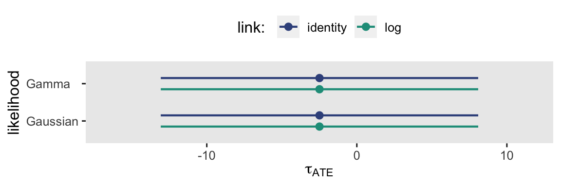
When you look at the results in the context of a plot like this, the subtle differences in their point estimates and 95% intervals seem trivial, don’t they? I don’t know that I can promise this will always be the case.

ANCOVA makes it hard.

If we once again use the conventional Gaussian likelihood with the identity link as a benchmark, our first ANCOVA-type model will follow the form

$$ \begin{align*} \text{post}_i & \sim \operatorname{Normal}(\mu_i, \sigma) \\ \mu_i & = \beta_0 + \beta_1 \text{experimental}_i + \beta_2 \text{prec}_i, \end{align*} $$

where \(\beta_2\) is the coefficient for our baseline covariate prec, which is the mean-centered version of the participant weights (in pounds) before the intervention.

Before we fit the models, we might want to make one more adjustment to the data. The prec covariate makes a lot of sense for the models using the identity link. However, it might make more sense to use a mean-centered version of the log of pre for the two models using the log link. That way, the pre- and post-intervention weights will both be on the same log scale in the model, and the covariate will still have that desirable mean center. We’ll call this new version of the variable prelc.

horan1971 <- horan1971 %>% 
  mutate(prelc = log(pre) - mean(log(pre)))

We might check to make sure both versions of the pre covariate have means at zero.

horan1971 %>% 
  pivot_longer(ends_with("c")) %>% 
  group_by(name) %>% 
  summarise(m = mean(value))

## # A tibble: 2 × 2
##   name          m
##   <chr>     <dbl>
## 1 prec  -8.67e-15
## 2 prelc -3.58e-16

Yep, they’re both zero within a very small rounding error.

Okay, here’s how to fit the ANCOVA-type models with the glm() function. As before, take special note of the family syntax.

# Gaussian, identity link
glm2a <- glm(
  data = horan1971,
  family = gaussian,
  post ~ 1 + experimental + prec)

# Gaussian, log link
glm2b <- glm(
  data = horan1971,
  family = gaussian(link = "log"),
  post ~ 1 + experimental + prelc)

# gamma, identity link
glm2c <- glm(
  data = horan1971,
  family = Gamma(link = "identity"),
  post ~ 1 + experimental + prec)

# gamma, log link
glm2d <- glm(
  data = horan1971,
  family = Gamma(link = "log"),
  post ~ 1 + experimental + prelc)

Check the model summaries.

summary(glm2a)

## 
## Call:
## glm(formula = post ~ 1 + experimental + prec, family = gaussian, 
##     data = horan1971)
## 
## Coefficients:
##               Estimate Std. Error t value Pr(>|t|)    
## (Intercept)  154.78354    1.36142 113.693   <2e-16 ***
## experimental  -4.57237    2.00226  -2.284   0.0281 *  
## prec           0.90845    0.05784  15.705   <2e-16 ***
## ---
## Signif. codes:  0 '***' 0.001 '**' 0.01 '*' 0.05 '.' 0.1 ' ' 1
## 
## (Dispersion parameter for gaussian family taken to be 40.69317)
## 
##     Null deviance: 11646.3  on 40  degrees of freedom
## Residual deviance:  1546.3  on 38  degrees of freedom
## AIC: 273.19
## 
## Number of Fisher Scoring iterations: 2

summary(glm2b)

## 
## Call:
## glm(formula = post ~ 1 + experimental + prelc, family = gaussian(link = "log"), 
##     data = horan1971)
## 
## Coefficients:
##               Estimate Std. Error t value Pr(>|t|)    
## (Intercept)   5.037021   0.008821 571.050   <2e-16 ***
## experimental -0.030434   0.013055  -2.331   0.0252 *  
## prelc         0.926027   0.058662  15.786   <2e-16 ***
## ---
## Signif. codes:  0 '***' 0.001 '**' 0.01 '*' 0.05 '.' 0.1 ' ' 1
## 
## (Dispersion parameter for gaussian family taken to be 40.53635)
## 
##     Null deviance: 11646.3  on 40  degrees of freedom
## Residual deviance:  1540.4  on 38  degrees of freedom
## AIC: 273.03
## 
## Number of Fisher Scoring iterations: 4

summary(glm2c)

## 
## Call:
## glm(formula = post ~ 1 + experimental + prec, family = Gamma(link = "identity"), 
##     data = horan1971)
## 
## Coefficients:
##               Estimate Std. Error t value Pr(>|t|)    
## (Intercept)  154.65699    1.35718 113.954   <2e-16 ***
## experimental  -4.31487    1.94553  -2.218   0.0326 *  
## prec           0.90019    0.05789  15.551   <2e-16 ***
## ---
## Signif. codes:  0 '***' 0.001 '**' 0.01 '*' 0.05 '.' 0.1 ' ' 1
## 
## (Dispersion parameter for Gamma family taken to be 0.001710954)
## 
##     Null deviance: 0.491977  on 40  degrees of freedom
## Residual deviance: 0.064439  on 38  degrees of freedom
## AIC: 271.51
## 
## Number of Fisher Scoring iterations: 4

summary(glm2d)

## 
## Call:
## glm(formula = post ~ 1 + experimental + prelc, family = Gamma(link = "log"), 
##     data = horan1971)
## 
## Coefficients:
##               Estimate Std. Error t value Pr(>|t|)    
## (Intercept)   5.036579   0.008808 571.811   <2e-16 ***
## experimental -0.029244   0.012951  -2.258   0.0298 *  
## prelc         0.917089   0.058234  15.748   <2e-16 ***
## ---
## Signif. codes:  0 '***' 0.001 '**' 0.01 '*' 0.05 '.' 0.1 ' ' 1
## 
## (Dispersion parameter for Gamma family taken to be 0.001704127)
## 
##     Null deviance: 0.491977  on 40  degrees of freedom
## Residual deviance: 0.064188  on 38  degrees of freedom
## AIC: 271.35
## 
## Number of Fisher Scoring iterations: 3

The way we interpret our \(\beta_1\) coefficients varies by model. For the Gaussian and gamma likelihoods, \(\beta_1\) is still an estimator of the ATE, but only when using the identity link function. Here they are:

bind_rows(
  tidy(glm2a, conf.int = TRUE), 
  tidy(glm2c, conf.int = TRUE)
) %>% 
  filter(term == "experimental") %>% 
  mutate(likelihood = likelihoods,
         link = rep(links, times = c(2, 0))) %>% 
  select(likelihood, link, estimate, std.error, starts_with("conf"))

## # A tibble: 2 × 6
##   likelihood link     estimate std.error conf.low conf.high
##   <chr>      <chr>       <dbl>     <dbl>    <dbl>     <dbl>
## 1 Gaussian   identity    -4.57      2.00    -8.50    -0.648
## 2 Gamma      identity    -4.31      1.95    -8.12    -0.498

Even though their numeric summaries are more notably different, now, both models’ version of \(\beta_1\) is still an estimator of the ATE. The estimators are just founded upon different distributional assumptions. Make your assumptions with care, friends.

The picture differs for the ANCOVA models using the log link. To my knowledge, there is no direct way to compute the ATE from their \(\beta_1\) coefficients, alone. The best we could do is use a combination of all three \(\beta\) coefficients and tricky exponentiation to compute some version of the CATE. But since the goal of this blog series is to focus on the ATE, we’ll avoid that kind of digression for now.

If we wanted to move away from interpreting the \(\beta\) coefficients directly, we can set the sole covariate to its mean value \((\bar c)\) to compute the conditional predicted values for the two levels of treatment, and then take their difference:

$$\tau_\text{ATE} = \mathbb E (y_i^1 \mid \bar c) - \mathbb E (y_i^0 \mid \bar c).$$

If we have more than one continuous covariate, we could generalize that equation so that \(\mathbf C_i\) is a vector of covariates, and update the equation for the ATE to account for our \(\mathbf{\bar C}\) vector to

$$\tau_\text{ATE} = \operatorname{\mathbb{E}} \left (y_i^1 \mid \mathbf{\bar C} \right) - \operatorname{\mathbb{E}} \left (y_i^0 \mid \mathbf{\bar C} \right).$$

This approach will only work, however, for our models which used the identity link. This will be a complete failure for the models which used the log link. Here we compute the results for all four models with predictions(), and reformat a little to make the output nicer.

# first set the predictor grid
nd <- tibble(experimental = 0:1,
             prec         = 0,
             prelc        = 0)

# compute
bind_rows(
  predictions(glm2a, newdata = nd, by = "experimental", hypothesis = "revpairwise"),
  predictions(glm2b, newdata = nd, by = "experimental", hypothesis = "revpairwise"),
  predictions(glm2c, newdata = nd, by = "experimental", hypothesis = "revpairwise"),
  predictions(glm2d, newdata = nd, by = "experimental", hypothesis = "revpairwise")
) %>% 
  data.frame() %>%
  mutate(likelihood = rep(likelihoods, each = 2) %>% factor(., levels = likelihoods),
         link = rep(links, times = 2) %>% factor(., levels = links),
         estimand = rep(c("ATE", "CATE"), times = 2)) %>% 
  select(likelihood, link, estimand, estimate, std.error, starts_with("conf")) %>%
  mutate_if(is.double, round, digits = 3)

##   likelihood     link estimand estimate std.error conf.low conf.high
## 1   Gaussian identity      ATE   -4.572     2.002   -8.497    -0.648
## 2   Gaussian      log     CATE   -4.616     1.978   -8.492    -0.741
## 3      Gamma identity      ATE   -4.315     1.946   -8.128    -0.502
## 4      Gamma      log     CATE   -4.437     1.963   -8.284    -0.589

This can be hard to catch because the differences among the estimates are all so subtle, but the results in the first and third rows are for the ATE, and the results in the second and fourth rows are for different versions of the CATE. The second row is the CATE for cases with a mean value for pre. The fourth row is the CATE for cases with a mean value for log-transformed pre. Here are what those mean values are on the pre scale.

horan1971 %>% 
  summarise(mean_pre = mean(pre),
            exponentiated_mean_log_pre = mean(log(pre)) %>% exp()) %>% 
  pivot_longer(everything())

## # A tibble: 2 × 2
##   name                       value
##   <chr>                      <dbl>
## 1 mean_pre                    155.
## 2 exponentiated_mean_log_pre  154.

Even though these look like integer values, that’s only because the output was rounded in the process of rendering this file into the format you see on the blog. Both summary numbers have a log trail of decimal digits.

Anyway, whether you’re using the Gaussian or gamma likelihood, you cannot use the \(\mathbb E (y_i^1 \mid \bar c) - \mathbb E (y_i^0 \mid \bar c)\) method to compute the ATE if you use the log link. If you prefer that method, you can only compute some version of the CATE.

Regardless of the link function, it’s the \(\mathbb E (y_i^1 - y_i^0 \mid c_i)\) method that will return an estimate for the ATE across ANCOVA-type models. That is, we compute each case’s \(y_i^1\) and \(y_i^0\) estimate, conditional on their baseline covariate value, take the difference in those estimates, and average across all cases. Before we do all that in one step with the handy avg_comparisons() function, it’s worth first showing the case-level predictions and their contrasts in a plot. Here are the case-level predictions from the four ANCOVA models.

# update the predictor grid to include all versions of the baseline covariate pre
nd <- horan1971 %>% 
  select(sn, prec, prelc, pre) %>% 
  expand_grid(experimental = 0:1)

# compute the counterfactual predictions for each case
bind_rows(
  predictions(glm2a, newdata = nd, by = c("sn", "experimental", "pre")),
  predictions(glm2b, newdata = nd, by = c("sn", "experimental", "pre")),
  predictions(glm2c, newdata = nd, by = c("sn", "experimental", "pre")),
  predictions(glm2d, newdata = nd, by = c("sn", "experimental", "pre"))
) %>% 
  # wrangle
  data.frame() %>% 
  mutate(y = ifelse(experimental == 0, "hat(italic(y))^0", "hat(italic(y))^1")) %>% 
  mutate(fit = rep(str_c("glm2", letters[1:4]), each = n() / 4)) %>% 
  mutate(likelihood = rep(likelihoods, each = n() / 2) %>% factor(., levels = likelihoods),
         link = rep(c(links, links), each = n() / 4) %>% factor(., levels = links)) %>% 
  
  # plot!
  ggplot(aes(x = estimate, y = reorder(sn, estimate))) +
  geom_interval(aes(xmin = conf.low, xmax = conf.high, color = y),
                    position = position_dodge(width = -0.2),
                    size = 1/5) +
  geom_point(aes(color = y, shape = y),
             size = 2) +
  scale_color_viridis_d(NULL, option = "A", begin = .3, end = .6,
                        labels = scales::parse_format()) +
  scale_shape_manual(NULL, values = c(20, 18),
              labels = scales::parse_format()) +
  scale_y_discrete(breaks = NULL) +
  labs(title = "Counterfactual predictions",
       x = "post",
       y = "sn (ranked)") +
  coord_cartesian(xlim = c(120, 200)) +
  theme(legend.background = element_blank(),
        legend.position = c(.9, .85)) +
  facet_grid(link ~ likelihood, labeller = label_both)

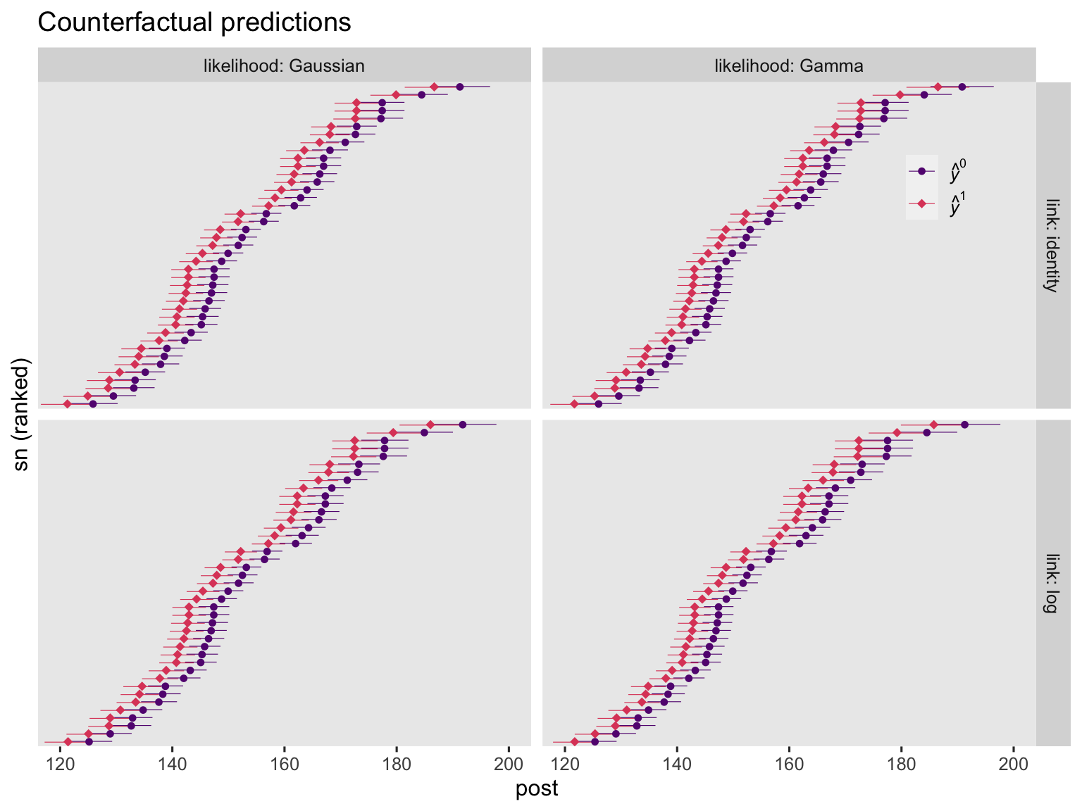
On the whole, the case-level counterfactual predictions are very similar across models. They aren’t exactly the same, though. This will be easier to see when we compare their contrasts.

bind_rows(
  comparisons(glm2a, variables = "experimental", by = "sn"),
  comparisons(glm2b, variables = "experimental", by = "sn"),
  comparisons(glm2c, variables = "experimental", by = "sn"),
  comparisons(glm2d, variables = "experimental", by = "sn")
) %>% 
  data.frame() %>% 
  mutate(fit = rep(str_c("glm2", letters[1:4]), each = n() / 4)) %>% 
  mutate(likelihood = rep(likelihoods, each = n() / 2) %>% factor(., levels = likelihoods),
         link = rep(c(links, links), each = n() / 4) %>% factor(., levels = links)) %>% 
  
  ggplot(aes(x = estimate, y = reorder(sn, estimate))) +
  geom_vline(xintercept = 0, color = "white") +
  geom_interval(aes(xmin = conf.low, xmax = conf.high),
                size = 1/5) +
  geom_point() +
  scale_y_discrete(breaks = NULL) +
  labs(title = "Treatment effects",
       x = expression(hat(tau)[italic(i)]~("i.e., "*hat(italic(y))[italic(i)]^1-hat(italic(y))[italic(i)]^0)),
       y = NULL) +
  xlim(-40, 40) +
  facet_grid(link ~ likelihood, labeller = label_both)

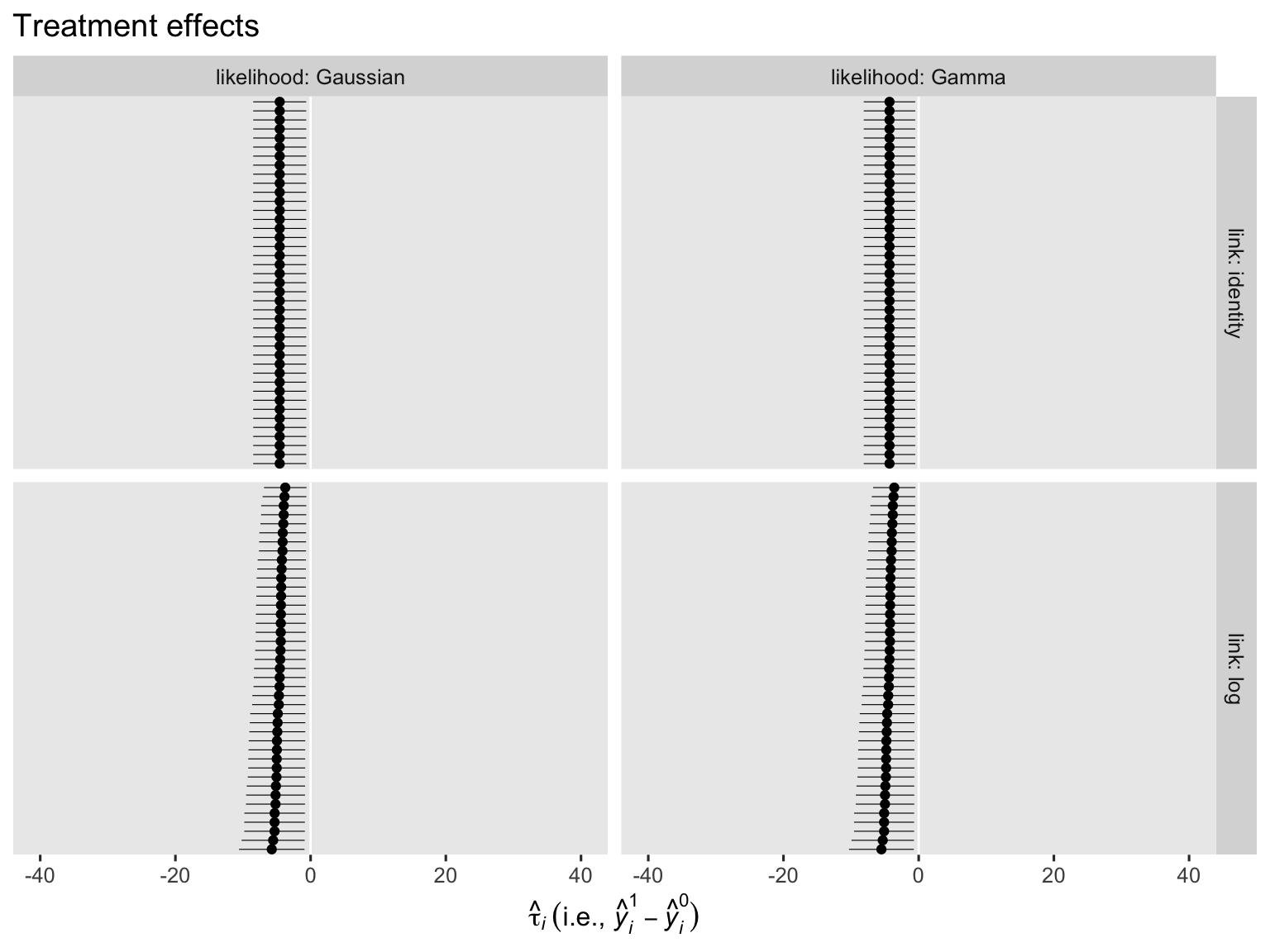
Regardless of the likelihood function, the models that used the identity link return identical \(\tau_i\) estimates for all cases. The log link, however, returned slightly different \(\tau_i\) estimates across the cases. The complication lies with the link function. Happily, all models return an estimate for \(\tau_\text{ATE}\) when we use the \(\mathbb E (y_i^1 - y_i^0 \mid c_i)\) method by way of the avg_comparisons() function.

bind_rows(
  avg_comparisons(glm2a, variables = "experimental"),
  avg_comparisons(glm2b, variables = "experimental"),
  avg_comparisons(glm2c, variables = "experimental"),
  avg_comparisons(glm2d, variables = "experimental")
) %>% 
  data.frame()%>%
  mutate(likelihood = rep(likelihoods, each = 2) %>% factor(., levels = likelihoods),
         link = rep(links, times = 2) %>% factor(., levels = links),
         estimand = "ATE") %>% 
  select(likelihood, link, estimand, estimate, std.error, starts_with("conf")) %>%
  mutate_if(is.double, round, digits = 3)

##   likelihood     link estimand estimate std.error conf.low conf.high
## 1   Gaussian identity      ATE   -4.572     2.002   -8.497    -0.648
## 2   Gaussian      log      ATE   -4.641     1.988   -8.538    -0.744
## 3      Gamma identity      ATE   -4.315     1.946   -8.128    -0.502
## 4      Gamma      log      ATE   -4.460     1.973   -8.328    -0.592

Even though the point estimates and their measures of uncertainty differ a bit, these are all estimators of the \(\tau_\text{ATE}\), each based on slightly different model assumptions. Here’s what they all look like in a coefficient plot.

bind_rows(
  avg_comparisons(glm2a, variables = "experimental"),
  avg_comparisons(glm2b, variables = "experimental"),
  avg_comparisons(glm2c, variables = "experimental"),
  avg_comparisons(glm2d, variables = "experimental")
) %>% 
  data.frame() %>% 
  mutate(likelihood = rep(likelihoods, each = 2) %>% factor(., levels = likelihoods),
         link = rep(links, times = 2) %>% factor(., levels = links)) %>% 

  ggplot(aes(x = estimate, xmin = conf.low, xmax = conf.high, y = likelihood, color = link)) +
  geom_pointinterval(position = position_dodge(width = -0.6),
                     linewidth = 2, point_size = 2) +
  scale_color_viridis_d("link: ", option = "D", begin = 0.25, end = 0.55, direction = 1) +
  scale_x_continuous(expression(tau[ATE]), expand = expansion(add = 5)) +
  theme(axis.text.y = element_text(hjust = 0),
        legend.position = "top")

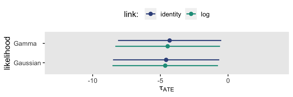
Which one is right? I can’t answer that for you. They’re all based on models with different underlying assumptions. Make your modeling assumptions with care, friends. Me, I like the gamma model with the log link.

Causal inference with Bayesian gamma regression

I’m not going to repeat all of our frequentist analyses as a Bayesian because that would make for an overly ponderous post. But I do think it’s reasonable to give a brief walk-through with a single Bayesian gamma ANCOVA model of the form

$$ \begin{align*} \text{post}_i & \sim \operatorname{Gamma}(\mu_i, \alpha) \\ \log(\mu_i) & = \beta_0 + \beta_1 \text{experimental}_i + \beta_2 \text{prelc}_i \\ \beta_0 & \sim \operatorname{Normal}(5.053056, 0.09562761) \\ \beta_1 & \sim \operatorname{Normal}(0, 0.25) \\ \beta_2 & \sim \operatorname{Normal}(0.75, 0.25) \\ \alpha & \sim \operatorname{Gamma}(0.01, 0.01). \end{align*} $$

Note that with brms, the gamma likelihood is parameterized in terms of the mean \((\mu)\) and the shape \((\alpha)\). If desired, we could compute the more familiar scale parameter \((\theta)\) with the equation

$$\theta = \frac{\mu}{\alpha}.$$

Anyway, my priors may look oddly specific. Let me walk them out.

Recall that in the fourth post, we used \(\operatorname{Normal}(156.5, 15)\) as the prior for the \(\beta_0\) intercept in the Gaussian model with the conventional identity link. Since we’re now using the log link, we need to set our priors with the conditional mean on the log scale. Did you know that if you take the log of a lognormal distribution, you end up with a normal distribution? The lognormal is a 2-parameter distribution over the positive real values, which has a nice right skew. The lognormal is odd in that its two parameters, \(\mu\) and \(\sigma\), are the population mean and standard deviation of the normal distribution you’d get after log-transforming the lognormal distribution. The math gets a little hairy, but if you wanted a lognormal distribution with a given mean and standard deviation on its own scale, you’d need to use the equations

$$ \begin{align*} \mu & = \log\left ( \bar y \Bigg / \sqrt{\frac{s^2}{\bar y^2} + 1} \right), \text{and} \\ \sigma & = \sqrt{\log \left(\frac{s^2}{\bar y^2} + 1 \right)}, \end{align*} $$

where \(\bar y\) is your desired mean and \(s\) is your desired SD. So what if we wanted a lognormal distribution that had a mean of 156.5 and a standard deviation of 15, to resemble the prior we used back in post #4? We could use those equations with the following code:

m <- 156.5  # desired mean
s <- 15     # desired SD

# use the equations
mu    <- log(m / sqrt(s^2 / m^2 + 1))
sigma <- sqrt(log(s^2 / m^2 + 1))

# what are the lognormal parameter values?
mu; sigma

## [1] 5.048484

## [1] 0.09562761

Here’s what that distribution looks like.

prior(lognormal(5.053056, 0.09562761)) %>% 
  parse_dist() %>% 
  
  ggplot(aes(xdist = .dist_obj, y = prior)) + 
  stat_halfeye(.width = c(.5, .95), p_limits = c(.0001, .9999)) +
  scale_y_discrete(NULL, breaks = NULL, expand = expansion(add = 0.1)) +
  labs(title = "Lognormal(5.053056, 0.09562761)",
       subtitle = "A normal prior on the log link is like a lognormal prior on the identity link.",
       x = expression(exp(italic(p)(beta[0])))) +
  coord_cartesian(xlim = c(100, 250))

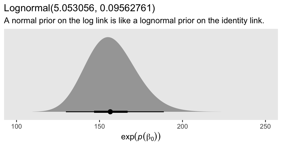
Thus, if we use a \(\operatorname{Normal}(5.053056, 0.09562761)\) prior for \(\beta_0\) on the log scale, that’s the equivalent of using a lognormal prior with a mean of 156.5 and a standard deviation of 15 on the identity scale.

Even though the \(\operatorname{Normal}(0, 0.25)\) prior might seem tight for our \(\beta_1\) coefficient for the group difference, keep in mind that difference is on the log scale. Thus, we’re putting about 95% of our prior mass on a half-log difference in either direction. For example, if we presume the control group will indeed have an average weight of 156.5 pounds, the \(\operatorname{Normal}(0, 0.25)\) prior puts 95% of the prior mass between these two weights for those in the experimental condition:

exp(5.053056 + c(-0.5, 0.5))

## [1]  94.92205 258.02488

That’s a wide spread, and frankly it suggests we could easily justify an even more conservative prior with a smaller value for the \(\sigma\) hyperparameter.

As to our \(\operatorname{Normal}(0.75, 0.25)\) prior for \(\beta_2\), this is suggesting the pre- and post-intervention weights scale close together, even when they’re on the log scale. In my experience, this is a good rule of thumb for behavioral data. If you’re not as confident as I am, adjust your prior accordingly.

The \(\operatorname{Gamma}(0.01, 0.01)\) prior for the shape parameter \(\alpha\) is the brm() default. You might use the get_prior() function to check this for yourself. If you’re going to be fitting a lot of Bayesian gamma regression models, you’re going to want to learn how to go beyond the default prior for your \(\alpha\) parameters. Since this is just a small point in a much larger story, I’m not going to dive much deeper into the topic, here. But if you wanted to start somewhere, keep in mind that when a gamma distribution’s \(\mu = \alpha\), the population mean and variance are the same;⁵ and with \(\mu\) held constant, larger values of \(\alpha\) make for smaller variances.⁶

Okay, here’s how to fit the model with brm().

# Bayesian gamma ANCOVA, with the log link
brm1 <- brm(
  data = horan1971,
  family = Gamma(link = "log"),
  post ~ 0 + Intercept + experimental + prelc,
  prior = prior(normal(5.053056, 0.09562761), class = b, coef = Intercept) +
    prior(normal(0, 0.25), class = b, coef = experimental) +
    prior(normal(0.75, 0.25), class = b, coef = prelc) +
    prior(gamma(0.01, 0.01), class = shape),  # the brms default
  cores = 4, seed = 6
)

Here we’ll compare the parameter summary for our Bayesian model to its maximum likelihood analogue.

summary(glm2d)  # maximum likelihood

## 
## Call:
## glm(formula = post ~ 1 + experimental + prelc, family = Gamma(link = "log"), 
##     data = horan1971)
## 
## Coefficients:
##               Estimate Std. Error t value Pr(>|t|)    
## (Intercept)   5.036579   0.008808 571.811   <2e-16 ***
## experimental -0.029244   0.012951  -2.258   0.0298 *  
## prelc         0.917089   0.058234  15.748   <2e-16 ***
## ---
## Signif. codes:  0 '***' 0.001 '**' 0.01 '*' 0.05 '.' 0.1 ' ' 1
## 
## (Dispersion parameter for Gamma family taken to be 0.001704127)
## 
##     Null deviance: 0.491977  on 40  degrees of freedom
## Residual deviance: 0.064188  on 38  degrees of freedom
## AIC: 271.35
## 
## Number of Fisher Scoring iterations: 3

print(brm1)  # Bayes via HMC

##  Family: gamma 
##   Links: mu = log; shape = identity 
## Formula: post ~ 0 + Intercept + experimental + prelc 
##    Data: horan1971 (Number of observations: 41) 
##   Draws: 4 chains, each with iter = 2000; warmup = 1000; thin = 1;
##          total post-warmup draws = 4000
## 
## Population-Level Effects: 
##              Estimate Est.Error l-95% CI u-95% CI Rhat Bulk_ESS Tail_ESS
## Intercept        5.04      0.01     5.02     5.06 1.00     2332     2462
## experimental    -0.03      0.02    -0.06     0.00 1.00     2348     2775
## prelc            0.91      0.06     0.78     1.03 1.00     3222     2591
## 
## Family Specific Parameters: 
##       Estimate Est.Error l-95% CI u-95% CI Rhat Bulk_ESS Tail_ESS
## shape   450.05    103.13   270.96   671.60 1.00     3284     2688
## 
## Draws were sampled using sampling(NUTS). For each parameter, Bulk_ESS
## and Tail_ESS are effective sample size measures, and Rhat is the potential
## scale reduction factor on split chains (at convergence, Rhat = 1).

The results for the \(\beta\) parameters are very similar.⁷

Since we’re in Bayesian mode, we might do a posterior-predictive check to make sure the model does an okay job simulating data that resemble the sample data.

set.seed(6)
pp_check(brm1, type = "dens_overlay_grouped", group = "experimental", ndraws = 100) +
  ggtitle("Posterior-predictive check (overlaid densities)")

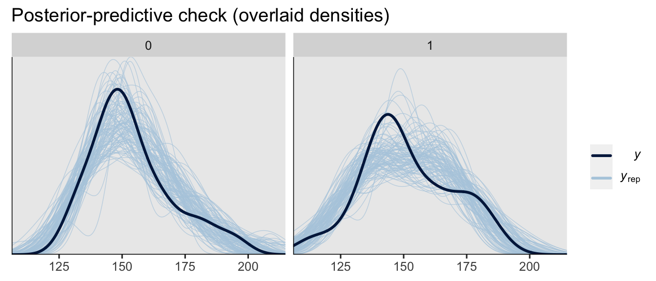
On the whole, the model did a pretty okay job capturing the skewed distributions of the original sample data. How’d we do capturing the conditional means, standard deviations and skewness, by experimental group?

set.seed(6)
p1 <- pp_check(brm1, type = "stat_grouped", group = "experimental", stat = "mean") +
  labs(subtitle = "Means") +
  coord_cartesian(xlim = c(143, 162))

set.seed(6)
p2 <- pp_check(brm1, type = "stat_grouped", group = "experimental", stat = "sd") +
  labs(subtitle = "SD's") +
  coord_cartesian(xlim = c(9, 26))

set.seed(6)
p3 <- pp_check(brm1, type = "stat_grouped", group = "experimental", stat = "skewness") +
  labs(subtitle = "Skews") +
  coord_cartesian(xlim = c(-1, 2))

# combine 
(p1 / p2 / p3) &
  theme(legend.position = "none") &
  plot_annotation(title = "Posterior-predictive statistical checks, by group",
                  subtitle = expression("The dark blue lines are "*italic(T(y))*", and the light blue bars are for "*italic(T)(italic(y)[rep])*"."))

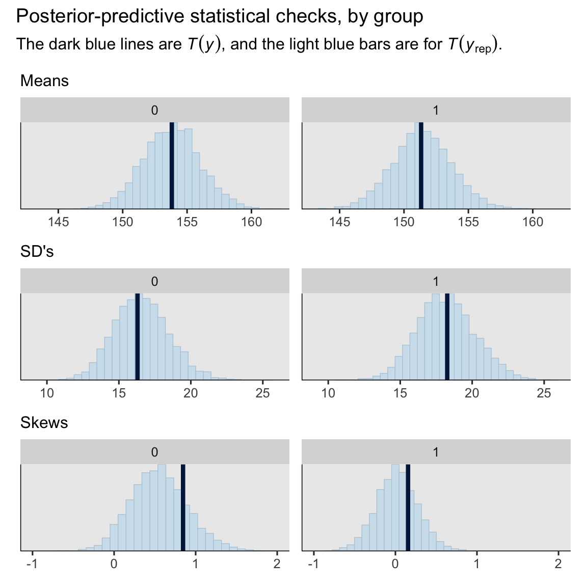
Our model did a great job with the means and SD’s, and a decent job with the skew.⁸

With our Bayesian gamma ANCOVA with the log link, the easiest way to compute our posterior for the ATE is with the avg_comparisons() function from marginaleffects.

avg_comparisons(brm1, variables = "experimental")

## 
##          Term Contrast Estimate 2.5 % 97.5 %
##  experimental    1 - 0    -4.48 -8.93  0.156
## 
## Columns: term, contrast, estimate, conf.low, conf.high

Recall that by default, the measure of central tendency in the Estimate column is the median for Bayesian models. If we wanted to get a look at the full posterior distribution for \(\tau_\text{ATE}\), we could tack on the posterior_draws() function from marginaleffects, and then plot or summarize as desired. Here’s what looks like for making a half-eye plot.

avg_comparisons(brm1, variables = "experimental") %>% 
   posterior_draws() %>% 
  
  ggplot(aes(x = draw)) +
  stat_halfeye(point_interval = mean_qi, .width = c(.5, .95)) +
  scale_y_continuous(NULL, breaks = NULL) +
  labs(title = "Bayesians like to show their posteriors.",
       x = expression(hat(tau)[ATE]))

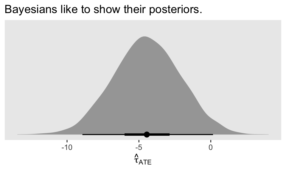
It’s a thing of beauty, isn’t it? For more details on how to use marginaleffects functions to work with brm() models, check out Arel-Bundock’s ( 2023) vignette, Bayesian analysis with brms. To see how to make the same computation with a fitted()- or add_epred_draws()-based workflow, go back to the fourth post in this series.

Recap

In this post, some of the main points we covered were:

• The gamma likelihood is a fine option for modeling right-skewed continuous variables with a lower limit of zero.
• The inverse function is the canonical link for gamma regression, but the log and identity links are popular alternatives.
• When you use the identity link for either the Gaussian or the gamma ANOVA, the \(\beta_1\) parameter, the \(\mathbb E (y_i^1 - y_i^0)\) method, and the \(\mathbb E (y_i^1) - \mathbb E (y_i^0)\) method are all valid estimators of \(\tau_\text{ATE}\).
• When you use the log link for either the Gaussian or the gamma ANOVA, only the \(\mathbb E (y_i^1 - y_i^0)\) method and the \(\mathbb E (y_i^1) - \mathbb E (y_i^0)\) method are all valid estimators of \(\tau_\text{ATE}\).
• When you use the identity link for either the Gaussian or the gamma ANCOVA, the \(\beta_1\) parameter, the \(\mathbb E (y_i^1 - y_i^0 \mid c_i)\) method, and the \(\mathbb E (y_i^1 \mid \bar c) - \mathbb E (y_i^0 \mid \bar c)\) method are all valid estimators of \(\tau_\text{ATE}\).
• When you use the log link for either the Gaussian or the gamma ANCOVA, only the \(\mathbb E (y_i^1 - y_i^0 \mid c_i)\) method can return a valid estimate for \(\tau_\text{ATE}\).

In the next post, we’ll explore how our causal inference methods work with ordinal regression models.

Thank the reviewer

I’d like to publicly acknowledge and thank

• Stephen J. Wild

for his kind efforts reviewing the draft of this post. Go team!

Do note the final editorial decisions were my own, and I do not think it would be reasonable to assume my reviewer has given a blanket endorsement of the current version of this post.

Session info

sessionInfo()

## R version 4.3.0 (2023-04-21)
## Platform: aarch64-apple-darwin20 (64-bit)
## Running under: macOS Ventura 13.4
## 
## Matrix products: default
## BLAS:   /Library/Frameworks/R.framework/Versions/4.3-arm64/Resources/lib/libRblas.0.dylib 
## LAPACK: /Library/Frameworks/R.framework/Versions/4.3-arm64/Resources/lib/libRlapack.dylib;  LAPACK version 3.11.0
## 
## locale:
## [1] en_US.UTF-8/en_US.UTF-8/en_US.UTF-8/C/en_US.UTF-8/en_US.UTF-8
## 
## time zone: America/Chicago
## tzcode source: internal
## 
## attached base packages:
## [1] stats     graphics  grDevices utils     datasets  methods   base     
## 
## other attached packages:
##  [1] patchwork_1.1.2        moments_0.14.1         brms_2.19.0            Rcpp_1.0.10           
##  [5] ggdist_3.3.0           marginaleffects_0.12.0 broom_1.0.5            lubridate_1.9.2       
##  [9] forcats_1.0.0          stringr_1.5.0          dplyr_1.1.2            purrr_1.0.1           
## [13] readr_2.1.4            tidyr_1.3.0            tibble_3.2.1           ggplot2_3.4.2         
## [17] tidyverse_2.0.0       
## 
## loaded via a namespace (and not attached):
##   [1] tensorA_0.36.2       rstudioapi_0.14      jsonlite_1.8.5       magrittr_2.0.3       TH.data_1.1-2       
##   [6] estimability_1.4.1   farver_2.1.1         nloptr_2.0.3         rmarkdown_2.22       vctrs_0.6.3         
##  [11] minqa_1.2.5          base64enc_0.1-3      blogdown_1.17        htmltools_0.5.5      distributional_0.3.2
##  [16] sass_0.4.6           StanHeaders_2.26.27  bslib_0.5.0          htmlwidgets_1.6.2    plyr_1.8.8          
##  [21] sandwich_3.0-2       emmeans_1.8.6        zoo_1.8-12           cachem_1.0.8         igraph_1.4.3        
##  [26] mime_0.12            lifecycle_1.0.3      pkgconfig_2.0.3      colourpicker_1.2.0   Matrix_1.5-4        
##  [31] R6_2.5.1             fastmap_1.1.1        collapse_1.9.6       shiny_1.7.4          digest_0.6.31       
##  [36] colorspace_2.1-0     ps_1.7.5             crosstalk_1.2.0      projpred_2.6.0       labeling_0.4.2      
##  [41] fansi_1.0.4          timechange_0.2.0     abind_1.4-5          mgcv_1.8-42          compiler_4.3.0      
##  [46] withr_2.5.0          backports_1.4.1      inline_0.3.19        shinystan_2.6.0      gamm4_0.2-6         
##  [51] pkgbuild_1.4.1       highr_0.10           MASS_7.3-58.4        gtools_3.9.4         loo_2.6.0           
##  [56] tools_4.3.0          httpuv_1.6.11        threejs_0.3.3        glue_1.6.2           callr_3.7.3         
##  [61] nlme_3.1-162         promises_1.2.0.1     grid_4.3.0           checkmate_2.2.0      reshape2_1.4.4      
##  [66] generics_0.1.3       gtable_0.3.3         tzdb_0.4.0           data.table_1.14.8    hms_1.1.3           
##  [71] utf8_1.2.3           pillar_1.9.0         markdown_1.7         posterior_1.4.1      later_1.3.1         
##  [76] splines_4.3.0        lattice_0.21-8       survival_3.5-5       tidyselect_1.2.0     miniUI_0.1.1.1      
##  [81] knitr_1.43           gridExtra_2.3        bookdown_0.34        stats4_4.3.0         xfun_0.39           
##  [86] bridgesampling_1.1-2 matrixStats_1.0.0    DT_0.28              rstan_2.21.8         stringi_1.7.12      
##  [91] yaml_2.3.7           boot_1.3-28.1        evaluate_0.21        codetools_0.2-19     cli_3.6.1           
##  [96] RcppParallel_5.1.7   shinythemes_1.2.0    xtable_1.8-4         munsell_0.5.0        processx_3.8.1      
## [101] jquerylib_0.1.4      coda_0.19-4          parallel_4.3.0       rstantools_2.3.1     ellipsis_0.3.2      
## [106] prettyunits_1.1.1    dygraphs_1.1.1.6     bayesplot_1.10.0     Brobdingnag_1.2-9    lme4_1.1-33         
## [111] viridisLite_0.4.2    mvtnorm_1.2-2        scales_1.2.1         xts_0.13.1           insight_0.19.2      
## [116] crayon_1.5.2         rlang_1.1.1          multcomp_1.4-24      shinyjs_2.1.0

References

Agresti, A. (2015). Foundations of linear and generalized linear models. John Wiley & Sons. https://www.wiley.com/en-us/Foundations+of+Linear+and+Generalized+Linear+Models-p-9781118730034
Arel-Bundock, V. (2023). Bayesian analysis with brms. https://vincentarelbundock.github.io/marginaleffects/articles/brms.html
Basu, A., Manning, W. G., & Mullahy, J. (2004). Comparing alternative models: Log vs Cox proportional hazard? Health Economics, 13(8), 749–765. https://doi.org/10.1002/hec.852
Bürkner, P.-C. (2023). Estimating distributional models with brms. https://CRAN.R-project.org/package=brms/vignettes/brms_distreg.html
Horan, J. J., & Johnson, R. G. (1971). Coverant conditioning through a self-management application of the Premack principle: Its effect on weight reduction. Journal of Behavior Therapy and Experimental Psychiatry, 2(4), 243–249. https://doi.org/10.1016/0005-7916(71)90040-1
Komsta, L., & Novomestky, F. (2022). Moments: Moments, cumulants, skewness, kurtosis and related tests [Manual]. https://CRAN.R-project.org/package=moments
Malehi, A. S., Pourmotahari, F., & Angali, K. A. (2015). Statistical models for the analysis of skewed healthcare cost data: A simulation study. Health Economics Review, 5(1), 1–16. https://doi.org/10.1186/s13561-015-0045-7
McCullagh, P., & Nelder, J. A. (1989). Generalized linear models (Second Edition). Chapman and Hall.
Nelder, J. A., & Wedderburn, R. W. (1972). Generalized linear models. Journal of the Royal Statistical Society: Series A (General), 135(3), 370–384. https://doi.org/10.2307/2344614
-
It isn’t totally under-used, though. Some researchers have found gamma regression (with the log link) useful for modeling healthcare cost data ( Basu et al., 2004; Malehi et al., 2015) ↩︎
We won’t entertain them all here, but gamma isn’t the only distribution in town that can describe non-negative, right-skewed, continuous data. Some of the alternatives include the exponential, inverse Gaussian, lognormal, and Weibull distributions. Fun fact: the exponential distribution can be thought of as a special case of the gamma distribution when the shape parameter of the gamma distribution
\((\alpha)\)is fixed to 1. Try it out and see. ↩︎ -
The language of “quirks” is my own. The inverse link has the technical limitation that it will not insure on its own that the model will not return negative predictions, which is an insight you can find in the technical literature (e.g., McCullagh & Nelder, 1989). In addition, I have personally found the inverse link can cause estimation difficulties with both frequentist (
glm()) and Bayesian (brm()) software. The log link just works, friends. Use the log link for gamma. ↩︎ -
You don’t have to believe me. Check it for yourself. You might do a visual check with a histogram or density plot. Or you could compute the sample skewness statistic with the
skewness()function from the moments package ( Komsta & Novomestky, 2022), which is what we’ll use in one of our posterior-predictive checks later on in the post. ↩︎ -
Why would I assume the mean and variance would be the same? you ask. Well, you might not. But bear in mind that the popular likelihood for unbounded counts, the Poisson, assumes the mean and variance are the same. Granted, the Poisson likelihood often underestimates the variance in real-world sample data, and we might not expect our positive-real skewed continuous data will behave like unbounded counts. But you have to start somewhere, friends. Why not appeal to one of the devils you already know? ↩︎
Within the context of a fixed
\(\mu\), you might think of\(\alpha\)as a concentration parameter. The higher the\(\alpha\), the more concentrated the distribution gets around the mean. ↩︎ -
Sharpe-eyed readers may have noticed that whereas the
glm()-based version of the model returned an estimate for a “dispersion” parameter, thebrm()-based model returned a posterior summary for a “shape” parameter. You may also have noticed that the estimate for the former is very small, and that the posterior mean for the latter is very large. What gives? Theglm()function parameterizes the gamma likelihood in terms of the mean\(\mu\)and dispersion\(\phi\), and the dispersion is just the inverse of the shape. That is\(\phi = 1 / \alpha\). ↩︎ -
I’ll admit, we did okay with the skew, but it seems like there’s room for improvement, particularly for the control condition. If you’re curious, try fitting a second Bayesian gamma model where you allow the log of the shape parameter
\((\log \alpha_i)\)to vary byexperimentalandprelc. I think you’ll see that fuller version of the model does a better job capturing the skew. We’re not quite ready for distributional models in this blog series, but check out Bürkner’s ( 2023) vignette, Estimating distributional models with brms, if you’re ready to skip ahead. ↩︎
- Posted on:
- May 14, 2023
- Length:
- 35 minute read, 7253 words