Causal inference with potential outcomes bootcamp

One of the nice things about the simple OLS models we fit in the last post is they’re easy to interpret. The various \(\beta\) parameters were valid estimates of the population effects for one treatment group relative to the wait-list control.¹ However, this nice property won’t hold in many cases where the nature of our dependent variables and/or research design requires us to fit other kinds of models from the broader generalized linear mixed model (GLMM) framework. Another issue at stake is if you’ve spent most of your statistical analysis career using the OLS framework, there’s a good chance there are concepts that are undifferentiated in your mind. As is turns out, some of these concepts are important when we want to make valid causal inferences. Our task in this post is to start differentiating the undifferentiated, by introducing some of the big concepts from the potential outcomes framework for causal inference.

Reload and refit

horan1971 data.

In post, we’ll be continuing on with our horan1971 data set form the last post. These data, recall, were transposed from the values displayed in Table 2 from Horan & Johnson ( 1971). I’ve saved them as an external .rda file on GitHub ( here). If you don’t want to download a data file from my GitHub, you can just copy the code from the last post.

# packages
library(tidyverse)
library(flextable)
library(marginaleffects)
library(ggdist)
library(patchwork)

# adjust the global theme
theme_set(theme_gray(base_size = 12) +
            theme(panel.grid = element_blank()))

# load the data from GitHub
load(url("https://github.com/ASKurz/blogdown/raw/main/content/blog/2023-04-12-boost-your-power-with-baseline-covariates/data/horan1971.rda?raw=true"))

# wrangle a bit
horan1971 <- horan1971 %>% 
  filter(treatment %in% c("delayed", "experimental")) %>% 
  mutate(prec = pre - mean(pre),
         experimental = ifelse(treatment == "experimental", 1, 0))

# what are these, again?
glimpse(horan1971)

## Rows: 41
## Columns: 8
## $ sl           <chr> "a", "b", "c", "d", "e", "f", "g", "h", "i", "j", "k", "l", "m", "n", "o", "p", "q", "r…
## $ sn           <int> 1, 2, 3, 4, 5, 6, 7, 8, 9, 10, 11, 12, 13, 14, 15, 16, 17, 18, 19, 20, 21, 22, 62, 63, …
## $ treatment    <fct> delayed, delayed, delayed, delayed, delayed, delayed, delayed, delayed, delayed, delaye…
## $ pre          <dbl> 149.50, 131.25, 146.50, 133.25, 131.00, 141.00, 145.75, 146.75, 172.50, 156.50, 153.00,…
## $ post         <dbl> 149.00, 130.00, 147.75, 139.00, 134.00, 145.25, 142.25, 147.00, 158.25, 155.25, 151.50,…
## $ prec         <dbl> -5.335366, -23.585366, -8.335366, -21.585366, -23.835366, -13.835366, -9.085366, -8.085…
## $ delayed      <dbl> 1, 1, 1, 1, 1, 1, 1, 1, 1, 1, 1, 1, 1, 1, 1, 1, 1, 1, 1, 1, 1, 1, 0, 0, 0, 0, 0, 0, 0, …
## $ experimental <dbl> 0, 0, 0, 0, 0, 0, 0, 0, 0, 0, 0, 0, 0, 0, 0, 0, 0, 0, 0, 0, 0, 0, 1, 1, 1, 1, 1, 1, 1, …

Same old models.

In the last post, we explored how to fit an ANOVA- and ANCOVA-type model to the data using OLS regression. For this post, we’ll refit those basic models. The ANOVA model for the data follows the form

$$ \begin{align*} \text{post}_i & = \beta_0 + \beta_1 \text{experimental}_i + \epsilon_i \\ \epsilon_i & \sim \operatorname{Normal}(0, \sigma), \end{align*} $$

where the two experimental conditions in play are captured by the dummy variable experimental. Here we fit that model again with the lm() function.

# fit the ANOVA model
ols1 <- lm(
  data = horan1971,
  post ~ experimental
)

# summarize the results
summary(ols1)

## 
## Call:
## lm(formula = post ~ experimental, data = horan1971)
## 
## Residuals:
##     Min      1Q  Median      3Q     Max 
## -36.829  -9.079  -4.818   9.932  40.182 
## 
## Coefficients:
##              Estimate Std. Error t value Pr(>|t|)    
## (Intercept)   153.818      3.674  41.864   <2e-16 ***
## experimental   -2.489      5.397  -0.461    0.647    
## ---
## Signif. codes:  0 '***' 0.001 '**' 0.01 '*' 0.05 '.' 0.1 ' ' 1
## 
## Residual standard error: 17.23 on 39 degrees of freedom
## Multiple R-squared:  0.005424,	Adjusted R-squared:  -0.02008 
## F-statistic: 0.2127 on 1 and 39 DF,  p-value: 0.6472

We also learned the ANCOVA model for these data follows the form

$$ \begin{align*} \text{post}_i & = \beta_0 + \beta_1 \text{experimental}_i + {\color{blueviolet}{\beta_2 \text{prec}_i}} + \epsilon_i \\ \epsilon_i & \sim \operatorname{Normal}(0, \sigma), \end{align*} $$

where \(\beta_2\) is the coefficient for our baseline covariate prec, which is the mean-centered version of the participant weights (in pounds) before the intervention. Here’s how to fit the ANCOVA-type model with lm().

# fit the ANCOVA model
ols2 <- lm(
  data = horan1971,
  post ~ 1 + experimental + prec
)

# summarize the results
summary(ols2)

## 
## Call:
## lm(formula = post ~ 1 + experimental + prec, data = horan1971)
## 
## Residuals:
##      Min       1Q   Median       3Q      Max 
## -12.5810  -3.3996  -0.4384   2.7288  13.9824 
## 
## Coefficients:
##               Estimate Std. Error t value Pr(>|t|)    
## (Intercept)  154.78354    1.36142 113.693   <2e-16 ***
## experimental  -4.57237    2.00226  -2.284   0.0281 *  
## prec           0.90845    0.05784  15.705   <2e-16 ***
## ---
## Signif. codes:  0 '***' 0.001 '**' 0.01 '*' 0.05 '.' 0.1 ' ' 1
## 
## Residual standard error: 6.379 on 38 degrees of freedom
## Multiple R-squared:  0.8672,	Adjusted R-squared:  0.8602 
## F-statistic: 124.1 on 2 and 38 DF,  p-value: < 2.2e-16

As expected, the \(\beta\) coefficients in the ANCOVA model all have smaller standard errors than those in the ANOVA model. Hurray! Statistics works!

Causal inference

Okay, so at the beginning of the post, we said the \(\beta\) coefficients for our experimental group are valid estimates of the population-level causal effects. But like, what does that even mean? Buckle up.

Counterfactual interventions, no covariates.

Our friends in causal inference have been busy over the past few years. First, we should understand there are different ways of speaking about causal inference. I’m not going to cover all the various frameworks, here, but most of the causal inference textbooks I mentioned in the last post provide historical overviews. At the time of this writing, I’m a fan of the potential-outcomes framework (see Imbens & Rubin, 2015; Rubin, 1974; Splawa-Neyman et al., 1990), the basics of which we might explain as follows:

Say you have some population of interest, such as overweight female university students interested in losing weight (see Horan & Johnson, 1971). You have some focal outcome variable \(y\), which you’d like to see change in a positive direction. In our case that would be bodyweight, as measured in pounds. Since \(y\) varies across \(i\) persons, we can denote each participants’ value as \(y_i\). Now imagine you have 2 or more well-defined interventions. In our case, that would be assignment to the waitlist control or experimental intervention group. For notation purposes, we can let \(0\) stand for the control group and \(1\) stand for the active treatment group, much like with a dummy variable. We can then write \(y_i^0\) for the \(i\)th person’s outcome if they were in the control condition, and \(y_i^1\) for the \(i\)th person’s outcome if they were in the treatment condition. Putting all those pieces together, we can define the causal effect \(\tau\) of treatment versus control for the \(i\)th person as

$$\tau_i = y_i^1 - y_i^0.$$

In the case of our horan1971 data, the causal effect of the experimental treatment for each woman is her post-treatment weight for the experimental treatment minus her post-treatment weight for the waitlist condition. The problem, however, is that each woman was only randomized into one of the two conditions. And thus, each woman has, at best, only 50% of the data required to compute her individual causal effect, \(\tau_i\). This is the so-called fundamental problem of causal inference ( Holland, 1986); we are always missing at least half of the data. To help illustrate this, take a look at a random subset of the horan1971 data.

set.seed(2)

horan1971 %>% 
  slice_sample(n = 10) %>% 
  mutate(y1 = ifelse(treatment == "experimental", post, NA),
         y0 = ifelse(treatment == "delayed", post, NA)) %>% 
  select(sn, treatment, post, y1, y0) %>% 
  flextable()

Within the mutate() function, I computed each participants’ y1 and y0 score, based on a combination of her treatment and post values. That last flextable() line converted the results to a nice table format, with help from the flextable package ( Gohel, 2023, 2022). Because none of the participants have values for both y1 and y0, we cannot use the raw data to compute their individual treatment effects. What we can do, however, is compute the average treatment effect (ATE) with the formula:

$$\tau_\text{ATE} = \mathbb E (y_i^1 - y_i^0),$$

which, in words, just means that the average treatment effect in the population is the same as the average of each person’s individual treatment effect. In the equation, I’m using the expectation operator \(\mathbb E()\) to emphasize we’re working within a likelihoodist framework. At first glance, it might appear² this equation doesn’t solve the problem that we cannot compute \(y_i^1 - y_i^0\) from the data of any of our participants, because half of the required values are still missing. However, it’s also the case that when we’re working with a simple OLS-type model,³

$$\tau_\text{ATE} = \mathbb E (y_i^1 - y_i^0) = {\color{blueviolet}{\mathbb E (y_i^1) - \mathbb E (y_i^0)}},$$

where \(\mathbb E (y_i^1)\) is the population average of our \(y_i^1\) values, and \(\mathbb E (y_i^0)\) is the population average of our \(y_i^0\) values. Even if if 50% of the values are missing, we can still compute \(\mathbb E (y_i^1)\), \(\mathbb E (y_i^0)\), and their difference.

Sometimes causal-inference scholars differentiate between the sample average treatment effect (SATE) and the population average treatment effect (PATE). In this blog post and in the rest of this series, I’m presuming y’all researchers are analyzing your data with regression models to make population-level inferences.⁴ Thus, I’m usually equating the ATE with the PATE. While I’m at it, there are other technical caveats which have to do with proper randomization and whether participants are truly independent of one another and so on. For the sake of this series, I’m presuming a clean simple randomization with no further complications. If you want more complications, check out Imbens & Rubin ( 2015) and any of the other texts on causal inference. Trust me, we have enough complications on our hands, as is.

Estimands, estimators, and estimates.

Before we get into it, we should probably introduce a few more vocabulary words.

• An estimand is the focal quantity of interest. It’s the reason we’re analyzing our data and it’s the answer to our primary research question. From a causal inference perspective, the estimand is the population-level causal effect.
• Estimators are the statistical methods we use to analyze our data. In this blog post and in the last, our estimators have been our OLS regression models. In the next couple blog posts, we’ll add logistic regression via maximum likelihood and various Bayesian models to our list of estimators.
• An estimate is the result from your statistical model (estimator) that’s designed to answer your research question.

Rubin ( 2005) did a pretty good job summarizing why terms like this are necessary:

When facing any problem of statistical inference, it is most important to begin by understanding the quantities that we are trying to estimate—the estimands. Doing so is particularly critical when dealing with causal inference, where mistakes can easily be made by describing the technique (e.g., computer program) used to do the estimation without any description of the object of the estimation. (p. 323)

I have made such mistakes, and my hope is this and the material to come will help prevent you from doing the same. If you prefer your education in the form of silly social media memes, maybe this one will help:

Was explaining the estimand/estimator/estimate distinction to a colleague earlier today and this meme came up so now you suffer too pic.twitter.com/7hhSMviuTj

— Richard McElreath 🦔 (@rlmcelreath) October 18, 2022

Anyway, next we’ll learn how to actually compute \(\tau_\text{ATE}\) within the context of our OLS models. This will be the estimate of our estimand.

Compute \(\mathbb E (y_i^1) - \mathbb E (y_i^0)\) from ols1.

Sometimes the authors of introductory causal inference textbooks have readers practice computing these values by hand, which can have its pedagogical value. But in your role as a professional scientist, you’ll be computing \(\tau_\text{ATE}\) within the context of a regression model so you can properly express the uncertainty of your estimate with 95% intervals, a standard error, or some other measure of uncertainty. To that end, we can compute \(\mathbb E (y_i^1)\) and \(\mathbb E (y_i^0)\) by inserting our ols1 model into the base R predict() function.

nd <- tibble(experimental = 0:1)

predict(ols1, 
        newdata = nd,
        se.fit = TRUE,
        interval = "confidence") %>% 
  data.frame() %>% 
  bind_cols(nd)

##    fit.fit  fit.lwr  fit.upr   se.fit df residual.scale experimental
## 1 153.8182 146.3863 161.2501 3.674259 39        17.2338            0
## 2 151.3289 143.3318 159.3261 3.953706 39        17.2338            1

The fit.fit column shows the point estimates, and the fit.lwr and fit.upr columns show the 95% intervals, and the se.fit columns shows the standard errors. Though the predict() method is great for computing \(\mathbb{E}(y_i^1)\) and \(\mathbb{E}(y_i^0)\), it doesn’t give us a good way to compute the difference of those values with a measure of uncertainty, such as a standard error. Happily, we can rely on functions from the handy marginaleffects package ( Arel-Bundock, 2023b) for that. First, notice how the predictions() function works in a similar way to the predict() function, but with nicer default behavior.

predictions(ols1, newdata = nd, by = "experimental")

## 
##  experimental Estimate Std. Error    z Pr(>|z|) 2.5 % 97.5 %
##             0      154       3.67 41.9   <0.001   147    161
##             1      151       3.95 38.3   <0.001   144    159
## 
## Columns: rowid, experimental, estimate, std.error, statistic, p.value, conf.low, conf.high, post

The marginaleffects package offers a few ways to contrast the two mean values. With the predictions() approach, we can just add in hypothesis = "revpairwise".

predictions(ols1, newdata = nd, by = "experimental", hypothesis = "revpairwise")

## 
##   Term Estimate Std. Error      z Pr(>|z|) 2.5 % 97.5 %
##  1 - 0    -2.49        5.4 -0.461    0.645 -13.1   8.09
## 
## Columns: term, estimate, std.error, statistic, p.value, conf.low, conf.high

Now we have a nice standard error and 95% interval for the estimate of our estimand \(\tau_\text{ATE}\). Thus, the average causal effect of the experimental condition relative to the waitlist control is a reduction of about 2 and a half pounds, with with a very wide 95% confidence interval spanning from a reduction of 13 pounds to an increase of 8 pounds. Now look back at the parameter summary for ols1.

summary(ols1)

## 
## Call:
## lm(formula = post ~ experimental, data = horan1971)
## 
## Residuals:
##     Min      1Q  Median      3Q     Max 
## -36.829  -9.079  -4.818   9.932  40.182 
## 
## Coefficients:
##              Estimate Std. Error t value Pr(>|t|)    
## (Intercept)   153.818      3.674  41.864   <2e-16 ***
## experimental   -2.489      5.397  -0.461    0.647    
## ---
## Signif. codes:  0 '***' 0.001 '**' 0.01 '*' 0.05 '.' 0.1 ' ' 1
## 
## Residual standard error: 17.23 on 39 degrees of freedom
## Multiple R-squared:  0.005424,	Adjusted R-squared:  -0.02008 
## F-statistic: 0.2127 on 1 and 39 DF,  p-value: 0.6472

Notice that the summary for our \(\beta_1\) parameter is the same as the estimate for \(\tau_\text{ATE}\) from above. When you have a simple OLS-type Gaussian model without a fancy link function, the estimate for \(\tau_\text{ATE}\) will be the same as the \(\hat \beta\) coefficient for the treatment dummy. As we will see in the next post, this will not generalize to other kinds generalized linear models (GLM’s).

Compute \(\mathbb E (y_i^1 - y_i^0)\) from ols1.

It’s time for me to confess my rhetoric above was a little misleading. As it turns out, you can in fact compute an estimate for \(\mathbb E (y_i^1 - y_i^0)\) from your regression models, even with 50% of the values missing. The key is to compute counterfactual estimates \(\hat y_i^1\) and \(\hat y_i^0\) from the model.⁵ Before we can do that, we’ll first need to redefine our nd predictor data.

nd <- horan1971 %>% 
  select(sn) %>% 
  expand_grid(experimental = 0:1)

# what?
glimpse(nd)

## Rows: 82
## Columns: 2
## $ sn           <int> 1, 1, 2, 2, 3, 3, 4, 4, 5, 5, 6, 6, 7, 7, 8, 8, 9, 9, 10, 10, 11, 11, 12, 12, 13, 13, 1…
## $ experimental <int> 0, 1, 0, 1, 0, 1, 0, 1, 0, 1, 0, 1, 0, 1, 0, 1, 0, 1, 0, 1, 0, 1, 0, 1, 0, 1, 0, 1, 0, …

What we’ve done is taken each unique case in the original horan1971 data, as indexed by sn, and assigned them both values for the experimental dummy, 0 and 1. As a consequence, we took our 41-row data frame and doubled it to 82 rows. Now we can insert our updated counterfactual nd data into the base R predict() function to compute all those \(\hat y_i^1\) and \(\hat y_i^0\) estimates.

predict(ols1, 
        newdata = nd,
        se.fit = TRUE,
        interval = "confidence") %>% 
  data.frame() %>% 
  bind_cols(nd) %>% 
  # just show the first 6 rows
  head()

##    fit.fit  fit.lwr  fit.upr   se.fit df residual.scale sn experimental
## 1 153.8182 146.3863 161.2501 3.674259 39        17.2338  1            0
## 2 151.3289 143.3318 159.3261 3.953706 39        17.2338  1            1
## 3 153.8182 146.3863 161.2501 3.674259 39        17.2338  2            0
## 4 151.3289 143.3318 159.3261 3.953706 39        17.2338  2            1
## 5 153.8182 146.3863 161.2501 3.674259 39        17.2338  3            0
## 6 151.3289 143.3318 159.3261 3.953706 39        17.2338  3            1

Now each case (sn) gets their own estimate for both levels of the experimental dummy. Given these are counterfactual estimates from a statistical model, they also come with their measures of uncertainty. But just like before, the predict() method doesn’t give us a good way to compute \(\mathbb E (y_i^1 - y_i^0)\) from those estimates in a way that accounts for the standard errors. Once again, the marginaleffects package has the solution. Like before, our first attempt will be to insert our updated nd data into the predictions() function. This time, we’ve included both the sn and experimental variables into the by argument, to help clarity the output.

predictions(ols1, newdata = nd, by = c("sn", "experimental")) %>% 
  head()

## 
##  sn experimental Estimate Std. Error    z Pr(>|z|) 2.5 % 97.5 %
##   1            0      154       3.67 41.9   <0.001   147    161
##   1            1      151       3.95 38.3   <0.001   144    159
##   2            0      154       3.67 41.9   <0.001   147    161
##   2            1      151       3.95 38.3   <0.001   144    159
##   3            0      154       3.67 41.9   <0.001   147    161
##   3            1      151       3.95 38.3   <0.001   144    159
## 
## Columns: rowid, sn, experimental, estimate, std.error, statistic, p.value, conf.low, conf.high, post

I’ve used the head() function to limit the output to the first six rows, but the full output would have all 82 rows worth of counterfactual predictions. Each one has its own standard error and so on. To compute the actual participant-level contrasts, \(y_i^1 - y_i^0\), we’ll want to switch to the marginaleffects::comparisons() function. Here we just need to use the variables argument to indicate we want counterfactual comparisons on the experimental dummy for each case in the original data set.

comparisons(ols1, variables = "experimental") %>% 
  head()

## 
##          Term Contrast Estimate Std. Error      z Pr(>|z|) 2.5 % 97.5 %
##  experimental    1 - 0    -2.49        5.4 -0.461    0.645 -13.1   8.09
##  experimental    1 - 0    -2.49        5.4 -0.461    0.645 -13.1   8.09
##  experimental    1 - 0    -2.49        5.4 -0.461    0.645 -13.1   8.09
##  experimental    1 - 0    -2.49        5.4 -0.461    0.645 -13.1   8.09
##  experimental    1 - 0    -2.49        5.4 -0.461    0.645 -13.1   8.09
##  experimental    1 - 0    -2.49        5.4 -0.461    0.645 -13.1   8.09
## 
## Columns: rowid, term, contrast, estimate, std.error, statistic, p.value, conf.low, conf.high, predicted, predicted_hi, predicted_lo, post, experimental

Here we see the \(\hat y_i^1 - \hat y_i^0\) contrast for the first six participants in the data set, each with its own standard errors and so on. To give you a better sense of what we’ve been computing, we might put the participant-level counterfactual predictions and their contrasts into a couple plots.

# counterfactual predictions
p1 <- predictions(ols1, newdata = nd, by = c("sn", "experimental")) %>% 
  data.frame() %>% 
  mutate(y = ifelse(experimental == 0, "hat(italic(y))^0", "hat(italic(y))^1")) %>% 
  
  ggplot(aes(x = estimate, y = reorder(sn, estimate), color = y)) +
  geom_interval(aes(xmin = conf.low, xmax = conf.high),
                position = position_dodge(width = -0.2),
                size = 1/5) +
  geom_point(aes(shape = y),
             size = 2) +
  scale_color_viridis_d(NULL, option = "A", begin = .3, end = .6,
                        labels = scales::parse_format()) +
  scale_shape_manual(NULL, values = c(20, 18),
                     labels = scales::parse_format()) +
  scale_y_discrete(breaks = NULL) +
  labs(subtitle = "Counterfactual predictions",
       x = "post",
       y = "sn (ranked)") +
  xlim(120, 200) +
  theme(legend.background = element_blank(),
        legend.position = c(.9, .85))

# treatment effects
p2 <- comparisons(ols1, variables = "experimental", by = "sn") %>% 
  data.frame() %>% 
  
  ggplot(aes(x = estimate, y = reorder(sn, estimate))) +
  geom_vline(xintercept = 0, color = "white") +
  geom_interval(aes(xmin = conf.low, xmax = conf.high),
                size = 1/5) +
  geom_point() +
  scale_y_discrete(breaks = NULL) +
  labs(subtitle = "Treatment effects",
       x = expression(hat(tau)[italic(i)]~("i.e., "*hat(italic(y))[italic(i)]^1-hat(italic(y))[italic(i)]^0)),
       y = NULL) +
  xlim(-40, 40)

# combine the two plots
p1 + p2 + plot_annotation(title = "Person-level estimates based on the ANOVA model (ols1)")

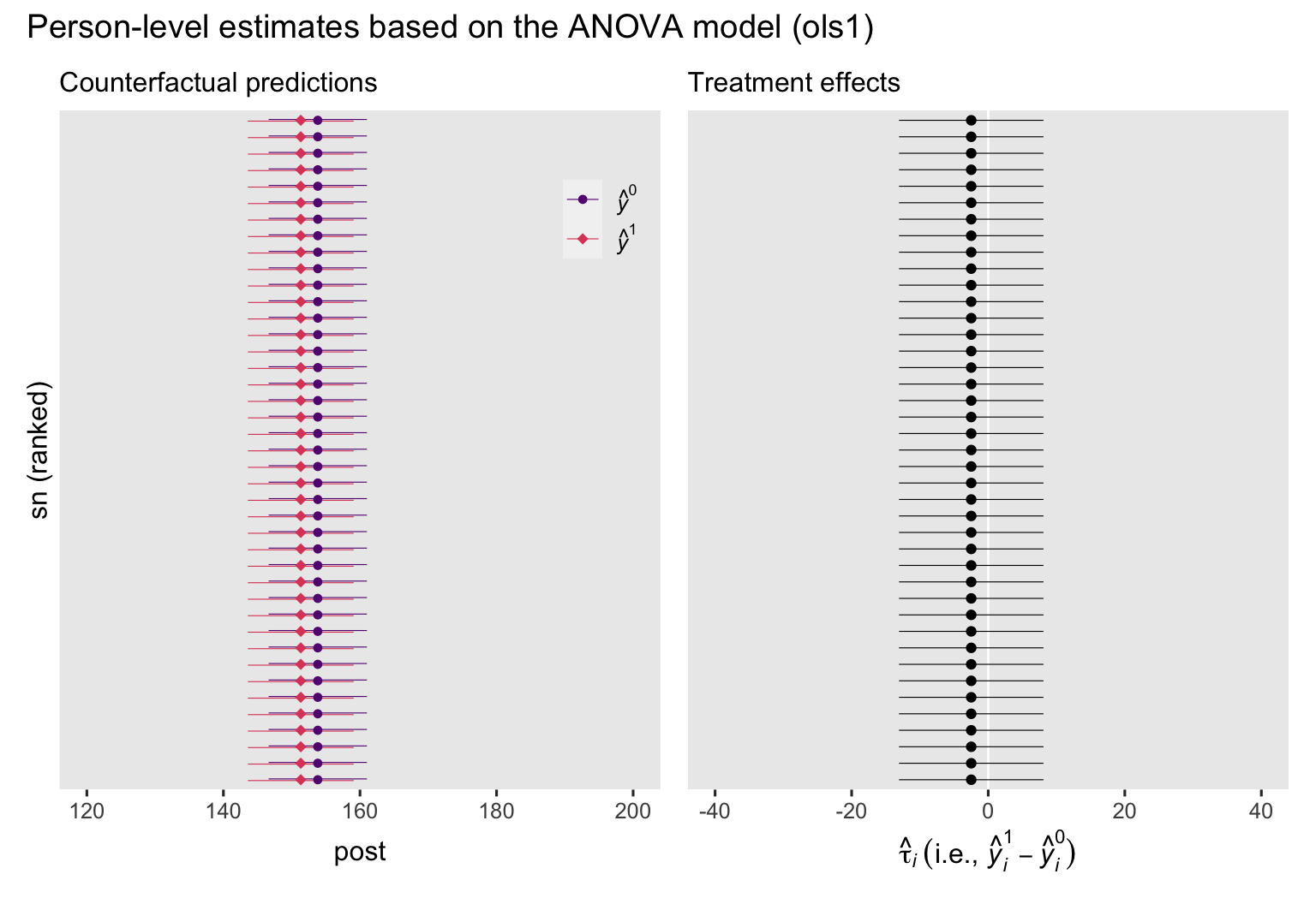
If the left plot, we see the counterfactual predictions, depicted by their point estimates (dots) and 95% intervals (horizontal lines), and colored by whether they were based on the waitlist group \((\hat y_i^0)\) or the experimental intervention \((\hat y_i^1)\). In the right plot, we have the corresponding treatment effects \((y_i^1 - y_i^0)\). In both plots, the y-axis has been rank ordered by the magnitudes of the predictions. Because the ANOVA model ols1 has no covariates, the predictions and their contrasts are identical for all participants, which makes rank ordering them an odd thing to do. As we’ll see later on, the ranking will make more sense once we work with the ANCOVA model.

But recall our focal estimand \(\tau_\text{ATE}\) is defined as \(\mathbb E (y_i^1 - y_i^0)\). This means we need a way to compute the average of those person-level contrasts, with a method that also accounts for their standard errors. Happily, all we need to do is use the summary() function after comparisons(), which will prompt the marginaleffects package to compute the average of those participant-level contrasts and use the so-called delta method to compute the accompanying standard error.

comparisons(ols1, variables = "experimental") %>% 
  summary()

## 
##          Term          Contrast Estimate Std. Error      z Pr(>|z|) 2.5 % 97.5 %
##  experimental mean(1) - mean(0)    -2.49        5.4 -0.461    0.645 -13.1   8.09
## 
## Columns: term, contrast, estimate, std.error, statistic, p.value, conf.low, conf.high

In this case our model-based estimate for \(\tau_\text{ATE}\), computed by the formula \(\mathbb E (y_i^1 - y_i^0)\), is the same as the \(\beta_1\) coefficient and its standard error. With a simple OLS-based ANOVA-type model of a randomized experiment,

• \(\beta_1\),
• \(\mathbb E (y_i^1 - y_i^0)\), and
• \(\mathbb E (y_i^1) - \mathbb E (y_i^0)\)

are all the same thing. They’re all estimators of our estimand \(\tau_\text{ATE}\), the average treatment effect.

Counterfactual interventions, with covariates.

Much like how we can use baseline covariates when we analyze RCT data to boost the power for \(\beta_1\), we can use baseline covariates when we make causal inferences, too. We just have to expand the framework a bit. If we let \(c_i\) stand for the \(i\)th person’s value on continuous covariate \(c\), we can estimate the ATE with help from covariate \(c\) with the formula:

$$\tau_\text{ATE} = \mathbb E (y_i^1 - y_i^0 \mid c_i),$$

which, in words, means that the average treatment effect in the population is the same as the average of each person’s individual treatment effect, computed conditional on their values of \(c\). We can generalize this equation so that \(\mathbf C_i\) is a vector of covariates, the values for which vary across the participants, to the following:

$$\tau_\text{ATE} = \mathbb E (y_i^1 - y_i^0 \mid \mathbf C_i).$$

Though we won’t consider more complex data examples in this blog post, we will want to keep the \(\mathbf C\) vector insights in the backs of our minds for the blog posts to come. In the literature, this method is often called standardization or g-computation. To my knowledge, these terms have their origins in different parts of the literature, but they’re really the same thing when used in the ways I’ll be highlighting in this blog series.⁶ For a way into this literature, you might check out Snowden et al. ( 2011), Muller & MacLehose ( 2014), or Wang et al. ( 2017).

Anyway, an alternative approach is to use the mean⁷ value of the covariate, \(\bar c\), to compute the conditional predicted values for the two levels of treatment, and then take their difference:

$$\tau_\text{ATE} = \mathbb E (y_i^1 \mid \bar c) - \mathbb E (y_i^0 \mid \bar c).$$

As above, we can generalize this equation so that \(\mathbf C_i\) is a vector of covariates, and update the equation for the ATE to account for our \(\mathbf{\bar C}\) vector to

$$\tau_\text{ATE} = \operatorname{\mathbb{E}} \left (y_i^1 \mid \mathbf{\bar C} \right) - \operatorname{\mathbb{E}} \left (y_i^0 \mid \mathbf{\bar C} \right).$$

As we will see, when working with a continuous outcome variable within the conventional OLS-type paradigm,

$$\mathbb E (y_i^1 - y_i^0 \mid c_i) = \mathbb E (y_i^1 \mid \bar c) - \mathbb E (y_i^0 \mid \bar c),$$

and

$$\mathbb E (y_i^1 - y_i^0 \mid \mathbf C_i) = \operatorname{\mathbb{E}} \left (y_i^1 \mid \mathbf{\bar C} \right) - \operatorname{\mathbb{E}} \left (y_i^0 \mid \mathbf{\bar C} \right).$$

In the next couple sections we’ll see what this looks like in action.

Compute \(\mathbb E (y_i^1 \mid \bar c) - \mathbb E (y_i^0 \mid \bar c)\) from ols2.

With our ANCOVA-type ols2 model, we can compute \(\mathbb E (y_i^1 \mid \bar c)\) and \(\mathbb E (y_i^0 \mid \bar c)\) with the base R predict() function. As a first step, we’ll define our prediction grid with the sample means for our covariate prec, and then expand the grid to include both values of the experimental dummy.

nd <- horan1971 %>% 
  summarise(prec = mean(prec)) %>% 
  expand_grid(experimental = 0:1)

# what?
print(nd)

## # A tibble: 2 × 2
##        prec experimental
##       <dbl>        <int>
## 1 -7.62e-15            0
## 2 -7.62e-15            1

In case you’re not used to scientific notation, the prec values in that output are basically zero. Since the prec covariate was already mean centered, we technically didn’t need to manually compute mean(prec); we already knew that value would be zero. But I wanted to make the point explicit so this step will generalize to other data contexts. Anyway, now we have our nd data, we’re ready to pump those values into predict().

predict(ols2, 
        newdata = nd,
        se.fit = TRUE,
        interval = "confidence") %>% 
  data.frame() %>% 
  bind_cols(nd)

##    fit.fit  fit.lwr  fit.upr   se.fit df residual.scale         prec experimental
## 1 154.7835 152.0275 157.5396 1.361421 38       6.379119 -7.62485e-15            0
## 2 150.2112 147.2450 153.1773 1.465200 38       6.379119 -7.62485e-15            1

Similar to the simple ANOVA-type ols1 version fo the model, the predict() method is great for computing \(\mathbb{E}(y_i^1 \mid \bar c)\) and \(\mathbb{E}(y_i^0 \mid \bar c)\), but it doesn’t give us a good way to compute the difference of those values with a measure of uncertainty. For that, we can once again rely on the marginaleffects::predictions() function.

predictions(ols2, newdata = nd, by = "experimental")

## 
##  experimental Estimate Std. Error   z Pr(>|z|) 2.5 % 97.5 %      prec
##             0      155       1.36 114   <0.001   152    157 -7.62e-15
##             1      150       1.47 103   <0.001   147    153 -7.62e-15
## 
## Columns: rowid, experimental, estimate, std.error, statistic, p.value, conf.low, conf.high, prec, post

To get the contrast, just add in hypothesis = "revpairwise".

predictions(ols2, newdata = nd, by = "experimental", hypothesis = "revpairwise")

## 
##   Term Estimate Std. Error     z Pr(>|z|) 2.5 % 97.5 %
##  1 - 0    -4.57          2 -2.28   0.0224  -8.5 -0.648
## 
## Columns: term, estimate, std.error, statistic, p.value, conf.low, conf.high

And also like with the ANOVA-type ols1, this method for computing the \(\tau_\text{ATE}\) from ols2 returns the same estimate and uncertainty statistics as returned by the summary() information for the \(\beta_1\) parameter.

summary(ols2)

## 
## Call:
## lm(formula = post ~ 1 + experimental + prec, data = horan1971)
## 
## Residuals:
##      Min       1Q   Median       3Q      Max 
## -12.5810  -3.3996  -0.4384   2.7288  13.9824 
## 
## Coefficients:
##               Estimate Std. Error t value Pr(>|t|)    
## (Intercept)  154.78354    1.36142 113.693   <2e-16 ***
## experimental  -4.57237    2.00226  -2.284   0.0281 *  
## prec           0.90845    0.05784  15.705   <2e-16 ***
## ---
## Signif. codes:  0 '***' 0.001 '**' 0.01 '*' 0.05 '.' 0.1 ' ' 1
## 
## Residual standard error: 6.379 on 38 degrees of freedom
## Multiple R-squared:  0.8672,	Adjusted R-squared:  0.8602 
## F-statistic: 124.1 on 2 and 38 DF,  p-value: < 2.2e-16

When you fit an OLS-type ANCOVA model with the conventional identity link, \(\mathbb{E}(y_i^1 \mid \bar c) - \mathbb{E}(y_i^0 \mid \bar c)\) will be the same as the \(\beta\) coefficient for the treatment dummy. They’re both estimators of our focal estimand \(\tau_\text{ATE}\).

Compute \(\mathbb E (y_i^1 - y_i^0 \mid c_i)\) from ols2.

Before we compute our counterfactual \(\mathbb{E}(y_i^1 - y_i^0 \mid c_i)\) estimates from our ANCOVA-type ols2, we’ll first need to redefine our nd predictor data. This time we’ll retain each participants’ prec value (i.e., \(c_i\)).

nd <- horan1971 %>% 
  select(sn, prec, pre) %>% 
  expand_grid(experimental = 0:1)

# what?
glimpse(nd)

## Rows: 82
## Columns: 4
## $ sn           <int> 1, 1, 2, 2, 3, 3, 4, 4, 5, 5, 6, 6, 7, 7, 8, 8, 9, 9, 10, 10, 11, 11, 12, 12, 13, 13, 1…
## $ prec         <dbl> -5.335366, -5.335366, -23.585366, -23.585366, -8.335366, -8.335366, -21.585366, -21.585…
## $ pre          <dbl> 149.50, 149.50, 131.25, 131.25, 146.50, 146.50, 133.25, 133.25, 131.00, 131.00, 141.00,…
## $ experimental <int> 0, 1, 0, 1, 0, 1, 0, 1, 0, 1, 0, 1, 0, 1, 0, 1, 0, 1, 0, 1, 0, 1, 0, 1, 0, 1, 0, 1, 0, …

Now each level of sn has two rows, one for each of the experimental dummy’s values: 0 and 1. But within each level of sn, the baseline covariate prec is held constant to its original value. Now we can insert our updated counterfactual nd into the base R predict() to compute the conditional estimates for post.

predict(ols2, 
        newdata = nd,
        se.fit = TRUE,
        interval = "confidence") %>% 
  data.frame() %>% 
  bind_cols(nd) %>% 
  # subset the output
  head()

##    fit.fit  fit.lwr  fit.upr   se.fit df residual.scale sn       prec    pre experimental
## 1 149.9366 147.1383 152.7349 1.382308 38       6.379119  1  -5.335366 149.50            0
## 2 145.3642 142.3035 148.4250 1.511950 38       6.379119  1  -5.335366 149.50            1
## 3 133.3573 129.5447 137.1700 1.883360 38       6.379119  2 -23.585366 131.25            0
## 4 128.7850 124.6350 132.9349 2.049955 38       6.379119  2 -23.585366 131.25            1
## 5 147.2112 144.3293 150.0932 1.423612 38       6.379119  3  -8.335366 146.50            0
## 6 142.6389 139.4715 145.8062 1.564584 38       6.379119  3  -8.335366 146.50            1

To keep the output simple, I used the head() function to display just the first six rows. With a little more wrangling, we can compute the point estimates for \((y_i^1 - y_i^0 \mid c_i)\).

predict(ols2, 
        newdata = nd,
        se.fit = TRUE,
        interval = "confidence") %>% 
  data.frame() %>% 
  bind_cols(nd) %>% 
  select(sn:experimental, fit.fit) %>% 
  pivot_wider(names_from = experimental, values_from = fit.fit) %>% 
  mutate(tau = `1` - `0`)

## # A tibble: 41 × 6
##       sn   prec   pre   `0`   `1`   tau
##    <int>  <dbl> <dbl> <dbl> <dbl> <dbl>
##  1     1  -5.34  150.  150.  145. -4.57
##  2     2 -23.6   131.  133.  129. -4.57
##  3     3  -8.34  146.  147.  143. -4.57
##  4     4 -21.6   133.  135.  131. -4.57
##  5     5 -23.8   131   133.  129. -4.57
##  6     6 -13.8   141   142.  138. -4.57
##  7     7  -9.09  146.  147.  142. -4.57
##  8     8  -8.09  147.  147.  143. -4.57
##  9     9  17.7   172.  171.  166. -4.57
## 10    10   1.66  156.  156.  152. -4.57
## # ℹ 31 more rows

Even though the participants vary on their point estimates for 0 and 1, they all have the same estimates for their difference, tau. This is a normal characteristic of analyses within the OLS-type paradigm, but it will not hold once we generalize to other kinds of likelihoods. You’ll see. But anyways, since this workflow won’t allow us to retain the uncertainty statistics, we’ll switch back to our marginaleffects-based workflow. As a first step, we insert our updated nd data into the predictions() function. This time we include the sn, experimental, and prec variables into the by argument, to help clarity the output.

predictions(ols2, newdata = nd, by = c("sn", "experimental", "prec")) %>% 
  head()

## 
##  sn experimental   prec Estimate Std. Error     z Pr(>|z|) 2.5 % 97.5 % pre
##   1            0  -5.34      150       1.38 108.5   <0.001   147    153 150
##   1            1  -5.34      145       1.51  96.1   <0.001   142    148 150
##   2            0 -23.59      133       1.88  70.8   <0.001   130    137 131
##   2            1 -23.59      129       2.05  62.8   <0.001   125    133 131
##   3            0  -8.34      147       1.42 103.4   <0.001   144    150 146
##   3            1  -8.34      143       1.56  91.2   <0.001   140    146 146
## 
## Columns: rowid, sn, experimental, prec, estimate, std.error, statistic, p.value, conf.low, conf.high, pre, post

The head() function to limited the output to the first six rows, but the full output would have all 82 rows worth of counterfactual predictions. Each one has its own standard error and so on. To compute the actual participant-level contrasts, \((y_i^1 - y_i^0 \mid c_i)\), we switch to the marginaleffects::comparisons() function. Here we just need to use the variables argument to indicate we want counterfactual comparisons on the two levels of the experimental dummy for each case in the original data set.

comparisons(ols2, variables = "experimental") %>% 
  head()

## 
##          Term Contrast Estimate Std. Error     z Pr(>|z|) 2.5 % 97.5 %
##  experimental    1 - 0    -4.57          2 -2.28   0.0224  -8.5 -0.648
##  experimental    1 - 0    -4.57          2 -2.28   0.0224  -8.5 -0.648
##  experimental    1 - 0    -4.57          2 -2.28   0.0224  -8.5 -0.648
##  experimental    1 - 0    -4.57          2 -2.28   0.0224  -8.5 -0.648
##  experimental    1 - 0    -4.57          2 -2.28   0.0224  -8.5 -0.648
##  experimental    1 - 0    -4.57          2 -2.28   0.0224  -8.5 -0.648
## 
## Columns: rowid, term, contrast, estimate, std.error, statistic, p.value, conf.low, conf.high, predicted, predicted_hi, predicted_lo, post, experimental, prec

Here we see the \((\hat y_i^1 - \hat y_i^0 \mid c_i)\) estimates for the first six participants in the data set, each with its own standard errors and so on. Like with the ANOVA model, we might put the participant-level counterfactual predictions and their contrasts into a couple plots to give you a better sense of what we’ve been computing.

# counterfactual predictions
p3 <- predictions(ols2, newdata = nd, by = c("sn", "experimental", "prec")) %>% 
  data.frame() %>% 
  mutate(y = ifelse(experimental == 0, "hat(italic(y))^0", "hat(italic(y))^1")) %>% 
  
  ggplot(aes(x = estimate, y = reorder(sn, estimate))) +
  geom_interval(aes(xmin = conf.low, xmax = conf.high, color = y),
                position = position_dodge(width = -0.2),
                size = 1/5) +
  geom_point(aes(color = y, shape = y),
             size = 2) +
  scale_color_viridis_d(NULL, option = "A", begin = .3, end = .6,
                        labels = scales::parse_format()) +
  scale_shape_manual(NULL, values = c(20, 18),
                     labels = scales::parse_format()) +
  scale_y_discrete(breaks = NULL) +
  labs(subtitle = "Counterfactual predictions",
       x = "post",
       y = "sn (ranked)") +
  coord_cartesian(xlim = c(120, 200)) +
  theme(legend.background = element_blank(),
        legend.position = c(.9, .85))

# treatment effects
p4 <- comparisons(ols2, variables = "experimental", by = "sn") %>% 
  data.frame() %>% 
  
  ggplot(aes(x = estimate, y = reorder(sn, estimate))) +
  geom_vline(xintercept = 0, color = "white") +
  geom_interval(aes(xmin = conf.low, xmax = conf.high),
                size = 1/5) +
  geom_point() +
  scale_y_discrete(breaks = NULL) +
  labs(subtitle = "Treatment effects",
       x = expression(hat(tau)[italic(i)]~("i.e., "*hat(italic(y))[italic(i)]^1-hat(italic(y))[italic(i)]^0)),
       y = NULL) +
  xlim(-40, 40)

# combine
p3 + p4 + plot_annotation(title = "Person-level estimates based on the ANCOVA model (ols2)")

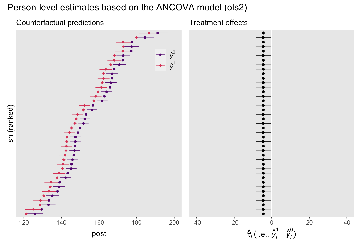
To my eye, a few things emerge when comparing these ANCOVA-based plots to their ANOVA counterparts from above. First, we now see how the prec covariate in the ANCOVA model changes the counterfactual predictions for the participants, and how each person’s predictions can vary widely from those for the other participants. Yet even though the individual predictions vary, the differences between \((\hat y_i^0)\) and \((\hat y_i^1)\) are the same across all participants, which is still depicted by the identical \(\hat \tau_i\) estimates in the right plot. Also, notice how the 95% intervals are much narrower in both plots, when compared to their ANOVA counterparts from above. This is why we like strongly-predictive baseline covariates. They shrink the standard errors and the 95% interval ranges.

But anyways, recall our focal estimand \(\tau_\text{ATE}\) is estimated via \(\mathbb E (\hat y_i^1 - \hat y_i^0 \mid c_i)\), which means we need to compute the average of those contrasts in a way that produces a standard error. As with the simpler ANOVA-type workflow we used with ols1, we can simply tack on a summary() line, which will compute delta-method based standard errors.⁸

comparisons(ols2, variables = "experimental") %>% 
  summary()

## 
##          Term          Contrast Estimate Std. Error     z Pr(>|z|) 2.5 % 97.5 %
##  experimental mean(1) - mean(0)    -4.57          2 -2.28   0.0224  -8.5 -0.648
## 
## Columns: term, contrast, estimate, std.error, statistic, p.value, conf.low, conf.high

When our goal is just to compute out estimate for \(\mathbb E (y_i^1 - y_i^0 \mid c_i)\), we can also use the marginaleffects::avg_comparisons() function, which skips the summary() step.

avg_comparisons(ols2, variables = "experimental")

## 
##          Term Contrast Estimate Std. Error     z Pr(>|z|) 2.5 % 97.5 %
##  experimental    1 - 0    -4.57          2 -2.28   0.0224  -8.5 -0.648
## 
## Columns: term, contrast, estimate, std.error, statistic, p.value, conf.low, conf.high

As Arel-Bundock pointed out his ( 2023a) vignette, Causal inference with the parametric g-formula, the avg_comparisons() function is a compact way to compute our estimate for \(\mathbb E (y_i^1 - y_i^0 \mid c_i)\) with the parametric g-formula method. Again in this case our estimate for \(\tau_\text{ATE}\) via \(\mathbb E (\hat y_i^1 - \hat y_i^0 \mid c_i)\) is the same as the \(\beta_1\) coefficient and its standard error from ols2, and they’re both the same as \(\tau_\text{ATE}\) estimated via the \(\mathbb E (\hat y_i^1 \mid \bar c) - \mathbb E (\hat y_i^0 \mid \bar c)\) method. We might further say that, in the case of an OLS-based ANCOVA-type model of a randomized experiment,

• \(\beta_1\),
• \(\mathbb{E}(y_i^1 - y_i^0 \mid c_i)\), and
• \(\mathbb{E}(y_i^1 \mid \bar c) - \mathbb{E}(y_i^0 \mid \bar c)\)

are all the same thing. They’re all equal to our estimand, the average treatment effect. We can extend this further to point out that the three estimators we used with our ANOVA-type model ols1 were also estimators of the average treatment effect. But the three methods we just used for our ANCOVA-type model ols2 all benefit from the increased precision (i.e., power) that comes from including a high-quality baseline covariate in the model.

But what about…?

When you want to estimate the ATE with covariates, our standardization/g-computation workflow isn’t the only workflow in town. Some of the noteworthy alternatives include inverse probability weighting and targeted maximum likelihood estimation. To fill my causal-inference needs, I’m looking for an approach with (a) good statistical properties (e.g., unbiased estimates), that (b) I can use as either a frequentist or a Bayesian, and will (c) apply to any number of models fit within the generalized linear mixed model framework and beyond (e.g., fully distributional models). At the moment, the standardization/g-computation approach seems to fit that bill, and we’ll get a better sense of this in later posts in this series. If you’d like to see a comparison of these various methods, check out the simulation study by Chatton et al. ( 2020).

Recap

In this post, some of the main points we covered were:

• The potential-outcomes framework is one of the contemporary approaches to causal inference.
• We cannot compute an individual’s causal effect \(\tau_i = y_i^1 - y_i^0\) by hand, because we are always missing at least half of the data. This is the fundamental problem of causal inference.
• Conceptually, the average treatment effect (ATE, \(\tau_\text{ATE}\)) is the mean of the person-specific treatment effects.
• In a simple ANOVA-type regression model, we can estimate \(\tau_\text{ATE}\) with either the \(\mathbb E (y_i^1 - y_i^0)\) or the \(\mathbb E (y_i^1) - \mathbb E (y_i^0)\) method, and the results will be exactly the same. Both methods will also be the same as the \(\beta\) coefficient for the treatment dummy in the ANOVA model.
• With an ANCOVA-type regression model with a single baseline covariate, we can estimate \(\tau_\text{ATE}\) with either the \(\mathbb E (y_i^1 - y_i^0 \mid c_i)\) or the \(\mathbb{E}(y_i^1 \mid \bar c) - \mathbb{E}(y_i^0 \mid \bar c)\) method, and the results will be exactly the same, granted we use the same covariate \(c\).
• We can generalize the two ANCOVA-type methods to models with multiple baseline covariates.

At this point, some readers might wonder why we have so many methods that produce the identical results. As we will soon see, this pattern will not generalize to models with other likelihoods and link functions. Speaking of which, in the next post we’ll see what this framework looks like for logistic regression.

Thank the reviewers

I’d like to publicly acknowledge and thank

• Chelsea M. Parlett-Pelleriti and
• Stephen J. Wild

for their kind efforts reviewing the draft of this post. Go team!

Do note the final editorial decisions were my own, and I do not think it would be reasonable to assume my reviewers have given blanket endorsements of the current version of this post.

Session information

sessionInfo()

## R version 4.2.3 (2023-03-15)
## Platform: x86_64-apple-darwin17.0 (64-bit)
## Running under: macOS Big Sur ... 10.16
## 
## Matrix products: default
## BLAS:   /Library/Frameworks/R.framework/Versions/4.2/Resources/lib/libRblas.0.dylib
## LAPACK: /Library/Frameworks/R.framework/Versions/4.2/Resources/lib/libRlapack.dylib
## 
## locale:
## [1] en_US.UTF-8/en_US.UTF-8/en_US.UTF-8/C/en_US.UTF-8/en_US.UTF-8
## 
## attached base packages:
## [1] stats     graphics  grDevices utils     datasets  methods   base     
## 
## other attached packages:
##  [1] patchwork_1.1.2             ggdist_3.2.1.9000           marginaleffects_0.11.1.9008
##  [4] flextable_0.9.1             lubridate_1.9.2             forcats_1.0.0              
##  [7] stringr_1.5.0               dplyr_1.1.2                 purrr_1.0.1                
## [10] readr_2.1.4                 tidyr_1.3.0                 tibble_3.2.1               
## [13] ggplot2_3.4.2               tidyverse_2.0.0            
## 
## loaded via a namespace (and not attached):
##  [1] fontquiver_0.2.1        insight_0.19.1.6        tools_4.2.3             backports_1.4.1        
##  [5] bslib_0.4.2             utf8_1.2.3              R6_2.5.1                colorspace_2.1-0       
##  [9] withr_2.5.0             tidyselect_1.2.0        curl_5.0.0              compiler_4.2.3         
## [13] textshaping_0.3.6       cli_3.6.1               xml2_1.3.3              officer_0.6.2          
## [17] fontBitstreamVera_0.1.1 labeling_0.4.2          bookdown_0.28           sass_0.4.5             
## [21] scales_1.2.1            checkmate_2.1.0         askpass_1.1             systemfonts_1.0.4      
## [25] digest_0.6.31           rmarkdown_2.21          gfonts_0.2.0            katex_1.4.0            
## [29] pkgconfig_2.0.3         htmltools_0.5.5         highr_0.10              fastmap_1.1.1          
## [33] rlang_1.1.0             rstudioapi_0.14         httpcode_0.3.0          shiny_1.7.2            
## [37] jquerylib_0.1.4         farver_2.1.1            generics_0.1.3          jsonlite_1.8.4         
## [41] zip_2.2.0               distributional_0.3.1    magrittr_2.0.3          Rcpp_1.0.10            
## [45] munsell_0.5.0           fansi_1.0.4             gdtools_0.3.3           lifecycle_1.0.3        
## [49] stringi_1.7.12          yaml_2.3.7              grid_4.2.3              promises_1.2.0.1       
## [53] crayon_1.5.2            hms_1.1.3               knitr_1.42              pillar_1.9.0           
## [57] uuid_1.1-0              crul_1.2.0              xslt_1.4.3              glue_1.6.2             
## [61] evaluate_0.20           blogdown_1.16           V8_4.2.1                fontLiberation_0.1.0   
## [65] data.table_1.14.8       vctrs_0.6.2             tzdb_0.3.0              httpuv_1.6.5           
## [69] gtable_0.3.3            openssl_2.0.6           cachem_1.0.7            xfun_0.39              
## [73] mime_0.12               xtable_1.8-4            later_1.3.0             equatags_0.2.0         
## [77] viridisLite_0.4.1       ragg_1.2.5              timechange_0.2.0        ellipsis_0.3.2

References

Arel-Bundock, V. (2023a). Causal inference with the parametric g-formula. https://vincentarelbundock.github.io/marginaleffects/articles/gformula.html
Arel-Bundock, V. (2023b). marginaleffects: Predictions, Comparisons, Slopes, Marginal Means, and Hypothesis Tests [Manual]. [https://vincentarelbundock.github.io/ marginaleffects/ https://github.com/vincentarelbundock/ marginaleffects]( https://vincentarelbundock.github.io/ marginaleffects/ https://github.com/vincentarelbundock/ marginaleffects)
Chatton, A., Le Borgne, F., Leyrat, C., Gillaizeau, F., Rousseau, C., Barbin, L., Laplaud, D., Léger, M., Giraudeau, B., & Foucher, Y. (2020). G-computation, propensity score-based methods, and targeted maximum likelihood estimator for causal inference with different covariates sets: A comparative simulation study. Scientific Reports, 10(1), 9219. https://doi.org/10.1038/s41598-020-65917-x
Gohel, D. (2023). Using the flextable R package. https://ardata-fr.github.io/flextable-book/
Gohel, D. (2022). flextable: Functions for tabular reporting [Manual]. https://CRAN.R-project.org/package=flextable
Hernán, M. A., & Robins, J. M. (2020). Causal inference: What if. Boca Raton: Chapman & Hall/CRC. https://www.hsph.harvard.edu/miguel-hernan/causal-inference-book/
Holland, P. W. (1986). Statistics and causal inference. Journal of the American Statistical Association, 81(396), 945–960. https://doi.org/ https://dx.doi.org/10.1080/01621459.1986.10478354
Horan, J. J., & Johnson, R. G. (1971). Coverant conditioning through a self-management application of the Premack principle: Its effect on weight reduction. Journal of Behavior Therapy and Experimental Psychiatry, 2(4), 243–249. https://doi.org/10.1016/0005-7916(71)90040-1
Imbens, G. W., & Rubin, D. B. (2015). Causal inference in statistics, social, and biomedical sciences: An Introduction. Cambridge University Press. https://doi.org/10.1017/CBO9781139025751
Keiding, N. (1987). The method of expected number of deaths, 1786-1886-1986, correspondent paper. International Statistical Review/Revue Internationale de Statistique, 55(1), 1–20. https://doi.org/10.2307/1403267
Lane, P. W., & Nelder, J. A. (1982). Analysis of covariance and standardization as instances of prediction. Biometrics. Journal of the International Biometric Society, 38(3), 613–621. https://doi.org/10.2307/2530043
Lin, W. (2013). Agnostic notes on regression adjustments to experimental data: Reexamining Freedman’s critique. 7(1), 295–318. https://doi.org/10.1214/12-AOAS583
Muller, C. J., & MacLehose, R. F. (2014). Estimating predicted probabilities from logistic regression: Different methods correspond to different target populations. International Journal of Epidemiology, 43(3), 962–970. https://doi.org/10.1093/ije/dyu029
Nelder, J. A., & Wedderburn, R. W. (1972). Generalized linear models. Journal of the Royal Statistical Society: Series A (General), 135(3), 370–384. https://doi.org/10.2307/2344614
Robins, J. (1986). A new approach to causal inference in mortality studies with a sustained exposure periodapplication to control of the healthy worker survivor effect. Mathematical Modelling, 7(9-12), 1393–1512. https://doi.org/10.1016/0270-0255(86)90088-6
Rubin, D. B. (1974). Estimating causal effects of treatments in randomized and nonrandomized studies. Journal of Educational Psychology, 66(5), 688–701. https://doi.org/10.1037/h0037350
Rubin, D. B. (2005). Causal inference using potential outcomes: Design, modeling, decisions. Journal of the American Statistical Association, 100(469), 322–331. https://doi.org/10.1198/016214504000001880
Snowden, J. M., Rose, S., & Mortimer, K. M. (2011). Implementation of G-computation on a simulated data set: Demonstration of a causal inference technique. American Journal of Epidemiology, 173(7), 731–738. https://doi.org/10.1093/aje/kwq472
Splawa-Neyman, J., Dabrowska, D. M., & Speed, T. P. (1990). On the Application of Probability Theory to Agricultural Experiments. Essay on Principles. Section 9. Statistical Science, 5(4), 465–472. https://doi.org/10.1214/ss/1177012031
Wang, A., Nianogo, R. A., & Arah, O. A. (2017). G-computation of average treatment effects on the treated and the untreated. BMC Medical Research Methodology, 17(3). https://doi.org/10.1186/s12874-016-0282-4
-
This, of course, is assuming you didn’t have major problems at the study design and implementation phases. If you did, those are issues for another blog series. ↩︎
I say “might appear” because we’ll eventually see this isn’t an unsolvable problem within our regression paradigm. But we do have to make some strong assumptions with our paradigm and the counterfactual estimates we’ll produce still aren’t the same thing as if we had actually observed all the potential outcomes. But we’re getting ahead of ourselves. ↩︎
As we’ll see later, this has a lot to do with link functions, which are popular with non-Gaussian models like logistic and Poisson regression. But basically, if you’re fitting a mean-model with an identity link, as with conventional OLS or a simple Gaussian GLM,
\(\mathbb E (y_i^1 - y_i^0) = \mathbb E (y_i^1) - \mathbb E (y_i^0)\). In other situations, it might not. ↩︎ -
A related issue is in some of the causal-inference literature (e.g., Lin, 2013; Splawa-Neyman et al., 1990), the authors have used a finite-population framework where the sample is the population. In this series, this will not be our approach. Rather, I am always assuming our sample is a representative subset of a superpopulation, as is typical in my field of psychology. ↩︎
Don Rubin isn’t a huge fan of equating counterfactuals with potential outcomes (see Rubin, 2005, p. 325). To my mind, this is the kind of nuanced distinction that may be of interest to philosophers or causal inference scholars, but has little importance for the kinds of applied statistical methods we’re highlighting in this series. ↩︎
I’m still getting my footing in this literature, so please forgive any mistakes in my documentation. To my knowledge, g-computation has its origins in the lengthy technical work by Robins ( 1986), an epidemiologist interested in causal inference with observational data. The practice of standardization (which does not mean computing
\(z\)scores in this context) has a long history among epidemiologist and demographers. For a historical and methodological overview of standardization for computing death rates within epidemiology, see Keiding ( 1987). I believe statisticians Lane and Nelder ( 1982) were the first to propose standardization as a post-processing step for ANCOVA-type GLM’s fit to data from experiments. Fun fact: Nelder was the principle author of, you know, the Generalized Linear Model ( Nelder & Wedderburn, 1972). No big deal. ↩︎ -
In addition to the sample mean, you could also use the mode (see Muller & MacLehose, 2014), or some other value of theoretical interest. The mode can be a particularly good option when working with categorical covariates, and we’ll cover this possibility in a future post. You could even use different strategies for different covariates in your covariate set. ↩︎
It’s a big deal how marginaleffects so easily returns standard errors and their derivatives (e.g., 95% CI’s,
\(p\)-values) for the\(\mathbb E (\hat y_i^1 - \hat y_i^0 \mid c_i)\)via the standardization/g-computation approach. Even pretty recent frequentist tutorials have relied on bootstrapping for standard errors and 95% intervals (e.g., Hernán & Robins, 2020; Wang et al., 2017). Bootstrapping methods are great in a pinch, but this is so much better. If you’d like to learn more, Arel-Bundock’s ( 2023a) vignette shows a comparison of the results from hisavg_comparisons()function to those from bootstrapping for one of the examples in Hernán and Robins’s ( 2020) textbook. ↩︎
- Posted on:
- April 16, 2023
- Length:
- 39 minute read, 8130 words