Causal inference with logistic regression

So far in this series, we’ve been been using ordinary least squares (OLS) to analyze and make causal inferences from our experimental data. Though OLS is an applied statistics workhorse and performs admirably in some cases, there are many contexts in which it’s just not appropriate. In medical trials, for example, many of the outcome variables are binary. Some typical examples are whether a participant still has the disease (coded 1) or not (coded 0), or whether a participant has died (coded 1) or is still alive (coded 0). In these cases, we want to model our data with a likelihood function that can handle binary data, and the go-to solution is the binomial.¹ As we will see, some of the nice qualities from the OLS paradigm fall apart when we want to make causal inferences with binomial models. But no fear; we have solutions.

We need data

In this post, we’ll be borrowing data from Wilson et al. ( 2017), Internet-accessed sexually transmitted infection (e-STI) testing and results service: A randomised, single-blind, controlled trial. Wilson and colleagues were open-science champions and made their primary data available as supporting information in a pmed.1002479.s001.xls file², which you can download by clicking this: https://doi.org/10.1371/journal.pmed.1002479.s001. ⚠️ For this next code block to work on your computer, you will need to first download that pmed.1002479.s001.xls file, and then save that file in a data subfolder in your working directory.

# packages
library(tidyverse)
library(marginaleffects)
library(flextable)
library(broom)
library(ggdist)
library(patchwork)

# adjust the global theme
theme_set(theme_gray(base_size = 12) +
            theme(panel.grid = element_blank()))

# load the data
wilson2017 <- readxl::read_excel("data/pmed.1002479.s001.xls", sheet = "data")

# what do these look like?
glimpse(wilson2017)

## Rows: 2,063
## Columns: 17
## $ anon_id     <dbl> 15005, 15008, 15013, 15015, 15018, 15022, 15024, 15030, 15031, 15037, 15039, 15040, 1504…
## $ group       <chr> "SH:24", "Control", "SH:24", "Control", "SH:24", "SH:24", "SH:24", "Control", "Control",…
## $ imd_decile  <dbl> 5, 6, 4, 2, 3, 2, 4, 2, 6, 2, 6, 3, 2, 4, 2, 3, 6, 4, 3, 3, 2, 6, 2, 3, 6, 3, 2, 4, 6, 4…
## $ partners    <chr> "3", "4", "3", "1", "2", "7", "4", "6", "6", "1", "3", "5", "3", "9", "1", "5", "3", "1"…
## $ gender      <chr> "Male", "Male", "Male", "Female", "Female", "Male", "Female", "Male", "Male", "Male", "F…
## $ msm         <chr> "other", "other", "other", "other", "other", "other", "other", "other", "msm", "other", …
## $ ethnicgrp   <chr> "Mixed/ Multiple ethnicity", "White/ White British", "Black/ Black British", "White/ Whi…
## $ age         <dbl> 27, 19, 26, 20, 24, 24, 24, 21, 24, 27, 21, 28, 24, 18, 26, 22, 23, 24, 26, 26, 22, 19, …
## $ anytest_sr  <dbl> 1, 0, 0, 0, 1, 1, 1, 0, NA, 1, 1, 1, 0, 1, 1, 1, 0, 1, 1, 1, 1, 1, 0, 1, 0, 1, 0, 1, 0, …
## $ anydiag_sr  <dbl> 0, 0, 0, 0, 0, 0, 0, 0, NA, 0, 0, 0, 0, 0, 0, 0, 0, 0, 0, 0, 0, 0, 0, 0, 0, 0, 0, 0, 0, …
## $ anytreat_sr <dbl> 0, 0, 0, 0, 0, 0, 0, 0, NA, 0, 0, 0, 0, 0, 0, 0, 0, 0, 0, 0, 0, 0, 0, 0, 0, 0, 0, 0, 0, …
## $ anytest     <dbl> 1, 0, 0, 0, 1, 1, 1, 0, NA, 0, 1, 0, 1, 0, 0, NA, 0, 0, 0, 1, 1, 1, 0, 0, 0, 1, 0, 1, 0,…
## $ anydiag     <dbl> 0, 0, 0, 0, 0, 0, 0, 0, NA, 0, 0, 0, 0, 0, 0, NA, 0, 0, 0, 0, 0, 0, 0, 0, 0, 0, 0, 0, 0,…
## $ anytreat    <dbl> 0, 0, 0, 0, 0, 0, 0, 0, NA, 0, 0, 0, 0, 0, 0, NA, 0, 0, 0, 0, 0, 0, 0, 0, 0, 0, 0, 0, 0,…
## $ time_test   <dbl> 33, 42, 42, 42, 7, 8, 18, 42, NA, 42, 10, 42, 31, 42, 42, NA, 42, 42, 42, 8, 4, 4, 42, 4…
## $ time_treat  <dbl> 84, 84, 84, 84, 84, 84, 84, 84, NA, 84, 84, 84, 84, 84, 84, NA, 84, 84, 84, 84, 84, 84, …
## $ sh24_launch <chr> "1 = dor post-launch", "0 = dor pre-launch", "1 = dor post-launch", "0 = dor pre-launch"…

These data were from a randomized controlled trial in London (2014–2015), which was designed to assess the effectiveness of an internet-accessed sexually transmitted infection testing (e-STI testing) and results service on STI testing uptake and STI cases diagnosed in chlamydia, gonorrhoea, HIV, and syphilis. The 2,072 participants were fluent in English, each had at least 1 sexual partner in the past year, consented to take an STI test, and had access to the internet. From the abstract, we further learn:

Participants were randomly allocated to receive 1 text message with the web link of an e-STI testing and results service (intervention group) or to receive 1 text message with the web link of a bespoke website listing the locations, contact details, and websites of 7 local sexual health clinics (control group). Participants were free to use any other services or interventions during the study period. The primary outcomes were self-reported STI testing at 6 weeks, verified by patient record checks, and self-reported STI diagnosis at 6 weeks, verified by patient record checks. (p. 1)

In the opening of the Results section (p. 8), we learn 9 more participants were excluded, leaving \(N = 2{,}063\) cases in the primary data set, which matches with the row number in the S1Data.xls data file. Here’s the count, by experimental condition.

wilson2017 %>% 
  count(group)

## # A tibble: 2 × 2
##   group       n
##   <chr>   <int>
## 1 Control  1032
## 2 SH:24    1031

For our analyses, we will take anytest as the focal variable. This variable indicates whether a participants’ medical record indicated any STI testing at 6 weeks. Here’s the breakdown, by experimental group.

wilson2017 %>% 
  count(group, anytest) %>% 
  group_by(group) %>% 
  mutate(percent_by_group = round(100 * n / sum(n), digits = 1))

## # A tibble: 6 × 4
## # Groups:   group [2]
##   group   anytest     n percent_by_group
##   <chr>     <dbl> <int>            <dbl>
## 1 Control       0   645             62.5
## 2 Control       1   173             16.8
## 3 Control      NA   214             20.7
## 4 SH:24         0   482             46.8
## 5 SH:24         1   439             42.6
## 6 SH:24        NA   110             10.7

As is often the case with real-world data, we have missing values. That could be fun problem with which to contend (see Bartlett et al., 2023), but that’s a task for another day. Walking out causal inference methods for a logistic regression paradigm will be a sufficient challenge, for now.

Subset.

The methods we’ll be exploring in this post will work perfectly fine with the full data set. But it’ll actually be easier for me to make some of my points if we reduce the sample size. Here we’ll take a random subset of \(n = 400\) of the cases with no missing data on the primary outcome variable anytest, and a few covariates of interest.

set.seed(1)

wilson2017 <- wilson2017 %>% 
  mutate(msm = ifelse(msm == 99, NA, msm)) %>% 
  drop_na(anytest, gender, partners, msm, ethnicgrp, age) %>% 
  slice_sample(n = 400)

# what are the dimensions?
dim(wilson2017)

## [1] 400  17

Now we’ll adjust some of the variables, themselves. We will save the nominal covariates gender, msm, and ethnicgrp as factors with defined levels. The covariate partners is ordinal,³ but for our purposes it will be fine to convert it to a factor, too. The age covariate is continuous, but it’ll come in handy to rescale it into a \(z\)-score metric, which we’ll name agez. We’ll simplify the character variable for the experimental groups, group, into a tx dummy coded 0 for the control condition and 1 for those in the intervention condition. Then we’ll rename the anon_id index to id, reorder the columns, and drop the other columns we won’t need for the rest of this post.

wilson2017 <- wilson2017 %>% 
  # factors
  mutate(gender    = factor(gender, levels = c("Female", "Male")),
         msm       = factor(msm, levels = c("other", "msm")),
         partners  = factor(partners, levels = c(1:9, "10+")),
         ethnicgrp = factor(ethnicgrp,
                            levels = c("White/ White British", "Asian/ Asian British", "Black/ Black British", "Mixed/ Multiple ethnicity", "Other"))) %>% 
  # z-score
  mutate(agez = (age - mean(age)) / sd(age)) %>% 
  # make a simple treatment dummy
  mutate(tx = ifelse(group == "SH:24", 1, 0)) %>% 
  # simplify the name
  rename(id = anon_id) %>% 
  # reorder and drop unneeded columns
  select(id, tx, anytest, gender, partners, msm, ethnicgrp, age, agez)

# what do we have?
glimpse(wilson2017)

## Rows: 400
## Columns: 9
## $ id        <dbl> 20766, 18778, 15678, 20253, 23805, 17549, 16627, 16485, 21905, 22618, 18322, 22481, 23708,…
## $ tx        <dbl> 0, 1, 0, 1, 0, 0, 1, 0, 0, 1, 1, 1, 1, 1, 1, 0, 0, 1, 0, 1, 1, 1, 1, 0, 1, 1, 1, 1, 0, 0, …
## $ anytest   <dbl> 0, 0, 0, 1, 1, 0, 0, 0, 0, 1, 0, 1, 0, 0, 1, 1, 0, 1, 0, 0, 0, 1, 0, 1, 1, 1, 0, 0, 0, 0, …
## $ gender    <fct> Male, Male, Female, Male, Female, Female, Male, Female, Male, Male, Female, Female, Male, …
## $ partners  <fct> 2, 4, 2, 1, 4, 2, 1, 2, 10+, 1, 1, 1, 1, 1, 2, 10+, 4, 10+, 1, 3, 1, 1, 1, 2, 3, 4, 3, 10+…
## $ msm       <fct> other, other, other, other, other, other, other, other, other, other, other, other, other,…
## $ ethnicgrp <fct> White/ White British, White/ White British, Mixed/ Multiple ethnicity, White/ White Britis…
## $ age       <dbl> 21, 19, 17, 20, 24, 19, 18, 20, 29, 28, 20, 23, 24, 24, 24, 20, 19, 27, 17, 23, 25, 23, 24…
## $ agez      <dbl> -0.53290527, -1.10362042, -1.67433557, -0.81826284, 0.32316745, -1.10362042, -1.38897799, …

Descriptive statistics

We’ve already introduced our binary outcome variable anytest and the experimental treatment dummy tx. In the paper’s Method section, we further learned the randomization algorithm balanced

for gender (male, female, transgender),⁴ age (16–19, 20–24, 25–30 years), number of sexual partners in last 12 months (1, 2+), and sexual orientation (MSM, all other groups). All factors had equal weight in determining marginal imbalance. (p. 4)

Further down in the Method (p. 7), we learn all these variables were used as covariates in the primary analysis,⁵ in addition to ethnicity.⁶

To get a sense of these covariates, we’ll make a Table 1 type table of the categorical variables for our randomized subset.

wilson2017 %>% 
  pivot_longer(cols = c(gender, partners, msm, ethnicgrp),
               names_to = "variable", values_to = "category") %>% 
  group_by(variable) %>% 
  count(category) %>% 
  mutate(`%` = round(100 * n / sum(n), digits = 1)) %>%
  as_grouped_data(groups = c("variable")) %>%
  flextable() %>%
  autofit() %>%
  italic(j = 3, part = "header")

Though we’ll be using the standardized version of age in the model, here are the basic descriptive statistics for age.

wilson2017 %>% 
  summarise(mean = mean(age),
            sd = sd(age),
            min = min(age),
            max = max(age))

## # A tibble: 1 × 4
##    mean    sd   min   max
##   <dbl> <dbl> <dbl> <dbl>
## 1  22.9  3.50    16    30

This was an RCT focusing on young adults.

Models

In this blog post, we’ll be fitting two models to these data. The first will be the unconditional ANOVA-type model

$$ \begin{align*} \text{anytest}_i & \sim \operatorname{Binomial}(n = 1, p_i) \\ \operatorname{logit}(p_i) & = \beta_0 + \beta_1 \text{tx}_i, \end{align*} $$

where \(\operatorname{logit}(.)\) indicates we’re using the conventional logit link.⁷ With this model, the experimental treatment dummy tx is the sole predictor of \(p_i\), on the log-odds scale. Then we’ll fit an ANCOVA-type version of the model including all the covariates:

$$ \begin{align*} \text{anytest}_i & \sim \operatorname{Binomial}(n = 1, p_i) \\ \operatorname{logit}(p_i) & = \beta_0 + \beta_1 \text{tx}_i \\ & \;\; + \beta_2 \text{agez}_i \\ & \;\; + \beta_3 \text{Male}_i \\ & \;\; + \beta_4 \text{MSM}_i \\ & \;\; + \beta_5 \text{Asian}_i + \beta_6 \text{Black}_i + \beta_7 \text{Mixed}_i + \beta_8 \text{Other}_i \\ & \;\; + \beta_9 \text{partners2}_i + \beta_{10} \text{partners3}_i + \dots + \beta_{17} \text{partners10}\texttt{+}_i, \end{align*} $$

where, due to the scoring of the covariates, the reference category would be a person in the control condition, who was of average age (22.9 years), a female not identifying as a man who slept with men, White, and who had been with one sexual partner over the past year. Here’s how to fit the models with the base R glm() function.

# ANOVA-type model
glm1 <- glm(
  data = wilson2017,
  family = binomial,
  anytest ~ tx
)

# ANCOVA-type model
glm2 <- glm(
  data = wilson2017,
  family = binomial,
  anytest ~ tx + agez + gender + msm + ethnicgrp + partners
)

# summarize the logistic-regression ANOVA
summary(glm1)

## 
## Call:
## glm(formula = anytest ~ tx, family = binomial, data = wilson2017)
## 
## Coefficients:
##             Estimate Std. Error z value Pr(>|z|)    
## (Intercept)  -1.1605     0.1672  -6.942 3.86e-12 ***
## tx            0.8728     0.2192   3.981 6.85e-05 ***
## ---
## Signif. codes:  0 '***' 0.001 '**' 0.01 '*' 0.05 '.' 0.1 ' ' 1
## 
## (Dispersion parameter for binomial family taken to be 1)
## 
##     Null deviance: 510.13  on 399  degrees of freedom
## Residual deviance: 493.74  on 398  degrees of freedom
## AIC: 497.74
## 
## Number of Fisher Scoring iterations: 4

# summarize the logistic-regression ANCOVA
summary(glm2)

## 
## Call:
## glm(formula = anytest ~ tx + agez + gender + msm + ethnicgrp + 
##     partners, family = binomial, data = wilson2017)
## 
## Coefficients:
##                                     Estimate Std. Error z value Pr(>|z|)    
## (Intercept)                         -1.35121    0.29151  -4.635 3.57e-06 ***
## tx                                   1.05449    0.23858   4.420 9.88e-06 ***
## agez                                 0.22252    0.12154   1.831   0.0671 .  
## genderMale                          -0.73481    0.29588  -2.483   0.0130 *  
## msmmsm                               0.32453    0.41020   0.791   0.4289    
## ethnicgrpAsian/ Asian British        0.06875    0.49533   0.139   0.8896    
## ethnicgrpBlack/ Black British       -0.17532    0.43259  -0.405   0.6853    
## ethnicgrpMixed/ Multiple ethnicity  -0.61378    0.41078  -1.494   0.1351    
## ethnicgrpOther                     -14.83385  670.96037  -0.022   0.9824    
## partners2                            0.21375    0.35314   0.605   0.5450    
## partners3                            0.72928    0.36598   1.993   0.0463 *  
## partners4                           -0.09513    0.43837  -0.217   0.8282    
## partners5                            1.09255    0.41769   2.616   0.0089 ** 
## partners6                            0.50061    0.59757   0.838   0.4022    
## partners7                            1.46416    0.66650   2.197   0.0280 *  
## partners8                            2.22407    1.12523   1.977   0.0481 *  
## partners9                           -0.09173    1.17444  -0.078   0.9377    
## partners10+                          0.51082    0.47750   1.070   0.2847    
## ---
## Signif. codes:  0 '***' 0.001 '**' 0.01 '*' 0.05 '.' 0.1 ' ' 1
## 
## (Dispersion parameter for binomial family taken to be 1)
## 
##     Null deviance: 510.13  on 399  degrees of freedom
## Residual deviance: 460.29  on 382  degrees of freedom
## AIC: 496.29
## 
## Number of Fisher Scoring iterations: 14

Note the parameter summary for ethnicgrpOther. Those values will come back to haunt us later in the post.

ATE for the ANOVA

As in our last blog post, our primary estimand will be the average treatment effect in the population, \(\tau_\text{ATE}\). However, we will cover a few alternative estimands along the way. We will begin by discussing the \(\beta\) coefficients and how they relate to our primary estimand \(\tau_\text{ATE}\).

\(\beta_1\) in the logistic regression ANOVA.

As a first step, let’s extract the \(\beta_1\) estimate from the ANOVA, with its standard error and so on, with help from the broom::tidy() function.

tidy(glm1, conf.int = T) %>% 
  filter(term == "tx")

## # A tibble: 1 × 7
##   term  estimate std.error statistic   p.value conf.low conf.high
##   <chr>    <dbl>     <dbl>     <dbl>     <dbl>    <dbl>     <dbl>
## 1 tx       0.873     0.219      3.98 0.0000685    0.447      1.31

The \(\beta_1\) parameter is on the log-odds scale, which isn’t the most intuitive, and can take some time to master. Though this won’t work for the standard error, test statistic and \(p\)-value, you can exponentiate the point estimate and 95% confidence intervals to convert those values to an odds-ratio metric.

tidy(glm1, conf.int = T) %>% 
  filter(term == "tx") %>% 
  select(estimate, starts_with("conf.")) %>% 
  mutate_all(exp)

## # A tibble: 1 × 3
##   estimate conf.low conf.high
##      <dbl>    <dbl>     <dbl>
## 1     2.39     1.56      3.70

Odds ratios range from 0 to positive infinity, and have an inflection point at 1. Though I don’t care for them, odds ratios seem to be popular effect sizes among medical researchers.⁸ To each their own. But if you’re like me, you want to convert the results of the model to the metric of a difference in probability.⁹ A naïve data analyst might try to convert \(\beta_1\) out of the log-odds metric into the probability metric with the base R plogis() function.

tidy(glm1, conf.int = T) %>% 
  filter(term == "tx") %>% 
  select(estimate, starts_with("conf.")) %>% 
  mutate_all(plogis)

## # A tibble: 1 × 3
##   estimate conf.low conf.high
##      <dbl>    <dbl>     <dbl>
## 1    0.705    0.610     0.787

This approach, however, DOES NOT convert \(\beta_1\) into a difference in probability. This is not an average treatment effect (ATE), and sadly, it’s completely uninterpretable. As Imbens and Ruben put it: “The average treatment effect cannot be expressed directly in terms of the parameters of the logistic or probit regression model” ( 2015, p. 128). But we can use an indirect method to compute the point estimate for the ATE with a combination of both \(\beta_0\) and \(\beta_1\), and the plogis() function.

plogis(coef(glm1)[1] + coef(glm1)[2]) - plogis(coef(glm1)[1])

## (Intercept) 
##   0.1899927

In somewhat awkward statistical notation, that code is

$$\operatorname{logit}^{-1}(\beta_0 + \beta_1) - \operatorname{logit}^{-1}(\beta_1),$$

where \(\operatorname{logit}^{-1}(\cdot)\) is the inverse of the logit function (i.e., plogis()).¹⁰ We can prove our estimate with this formula is correct by comparing it to the sample ATE (SATE), as computed by hand with sample statistics.

wilson2017 %>% 
  group_by(tx) %>% 
  summarise(p = mean(anytest == 1)) %>% 
  pivot_wider(names_from = tx, values_from = p) %>% 
  mutate(sate = `1` - `0`)

## # A tibble: 1 × 3
##     `0`   `1`  sate
##   <dbl> <dbl> <dbl>
## 1 0.239 0.429 0.190

Unlike with OLS-type models, you cannot estimate the ATE in a logistic-regression context with \(\beta_1\) alone. You need to account for the other parameters in the model, too. This is a pattern we’ll see again and again throughout this blog series.

Compute \(\Pr (y_i^1 = 1) - \Pr(y_i^0 = 1)\) from glm1.

Back in the last post, we leaned we could compute our primary causal estimand, the average treatment effect \(\tau_\text{ATE}\), in two ways:

$$\tau_\text{ATE} = \mathbb E (y_i^1 - y_i^0) = \mathbb E (y_i^1) - \mathbb E (y_i^0),$$

where, for the moment, we’re excluding covariates from the framework. As it turns out, these equalities hold regardless of whether \(y_i\) is of a continuous or binary variable. If we focus on the second method, \(\mathbb E (y_i^1)\) and \(\mathbb E (y_i^0)\) are probabilities for binary variables. To walk that out in statistical notation,

$$ \begin{align*} \mathbb E (y_i^1) & = {\color{blueviolet}{\Pr (y_i^1 = 1)}}\ \text{and} \\ \mathbb E (y_i^0) & = {\color{blueviolet}{\Pr (y_i^0 = 1)}}, \end{align*} $$

which means that

$$\mathbb E (y_i^1) - \mathbb E (y_i^0) = \Pr (y_i^1 = 1) - \Pr(y_i^0 = 1).$$

To take the notation even further, we typically use \(p\) in place of \(\Pr()\) when working with models fit with the binomial likelihood. Therefore

$$ \begin{align*} \mathbb E (y_i^1) & = \Pr (y_i^1 = 1) = {\color{blueviolet}{p^1}}\ \text{and} \\ \mathbb E (y_i^0) & = \Pr (y_i^0 = 1) = {\color{blueviolet}{p^0}}, \end{align*} $$

and finally

$$ \begin{align*} \mathbb E (y_i^1) - \mathbb E (y_i^0) & = \Pr (y_i^1 = 1) - \Pr(y_i^0 = 1) \\ & = p^1 - p^0. \end{align*} $$

This is all important because within the context of our binomial regression model, we can compute the population estimates for \(p^1\), \(p^0\), and their difference. Thus in the case of the binomial ANOVA model,

$$\tau_\text{ATE} = p^1 - p^0.$$

If you just wanted to compute the contrast between the two group-level probabilities, the base R predict() approach might be a good place to start. Here we define a simple data frame with the two levels of the tx dummy, and pump those values into predict().

nd <- tibble(tx = 0:1)

# log odds metric
predict(glm1, 
        newdata = nd,
        se.fit = TRUE) %>% 
  data.frame() %>% 
  bind_cols(nd)

##          fit    se.fit residual.scale tx
## 1 -1.1604877 0.1671622              1  0
## 2 -0.2876821 0.1418272              1  1

Note how the default behavior is to return the estimates and their standard errors in the log-odds metric. Also note that when working with binomial models, predict() will not return 95% confidence intervals. If you want the estimate in the probability metric, you can set type = "response".

# probability metric
predict(glm1, 
        newdata = nd,
        se.fit = TRUE,
        type = "response") %>% 
  data.frame() %>% 
  bind_cols(nd)

##         fit     se.fit residual.scale tx
## 1 0.2385787 0.03036651              1  0
## 2 0.4285714 0.03473318              1  1

And just to check, here’s how those estimates match up with the sample statistics.

wilson2017 %>% 
  group_by(tx) %>% 
  summarise(p = mean(anytest == 1))

## # A tibble: 2 × 2
##      tx     p
##   <dbl> <dbl>
## 1     0 0.239
## 2     1 0.429

However, this approach gives us no way to compute the contrast of those probabilities in a way that retains the uncertainty information in the standard errors. For that, we turn once again to the marginaleffects package. To start, we can use the predictions() function to return the group probabilities, along with their measures of uncertainty.

predictions(glm1, newdata = nd, by = "tx")

## 
##  tx Estimate Pr(>|z|) 2.5 % 97.5 %
##   0    0.239   <0.001 0.184  0.303
##   1    0.429   0.0425 0.362  0.498
## 
## Columns: rowid, tx, estimate, p.value, conf.low, conf.high, anytest

Notice how predictions() returns probabilities by default, rather than log odds. To get the contrast for the two probabilities, just add hypothesis = "revpairwise".

predictions(glm1, newdata = nd, by = "tx", hypothesis = "revpairwise")

## 
##   Term Estimate Std. Error    z Pr(>|z|)  2.5 % 97.5 %
##  1 - 0     0.19     0.0461 4.12   <0.001 0.0996   0.28
## 
## Columns: term, estimate, std.error, statistic, p.value, conf.low, conf.high

Not only do we get the probability contrast, but we get the standard error and confidence intervals, too. That, friends, if our first estimate of \(\tau_\text{ATE}\) from a logistic regression model.

Compute \(\mathbb E (p_i^1 - p_i^0)\) from glm1.

Within the context of our ANOVA-type binomial model, the \(\mathbb E (y_i^1 - y_i^0)\) method still works fine for estimating the ATE. But there are new conceptual quirks with which we must contend. First, unlike with continuous variables, there are only four possible combinations of \(y_i^1\) and \(y_i^0\), and there are only three possible values for \(\tau_i\).

crossing(y0 = 0:1, 
         y1 = 0:1) %>% 
  mutate(tau = y1 - y0) %>%
  flextable()

Imbens and Rubin discussed this kind of scenario in Section 1.3 in their ( 2015) text. If we were in a context where we could compute the raw \(y_i^1 - y_i^0\) contrasts with synthetic data, the average of those values,

$$\tau_\text{SATE} = \frac{1}{N} \sum_{i=1}^N (y_i^1 - y_i^0),$$

could take on any continuous value ranging from -1 to 1. Thus unlike with the OLS paradigm for continuous variables, the metric for \(\tau_\text{SATE}\), and also \(\tau_\text{ATE}\), is not the same as the metric for any individual case’s causal effect \(\tau_i\). The average of a set of integers is a real number.

The second issue is when we compute the case-specific counterfactual estimates from a logistic regression model, we don’t typically get a vector of \(\hat y_i^1\) and \(\hat y_i^1\) values; we get \(\hat p_i^1\) and \(\hat p_i^0\) instead. Let’s explore what that looks like with predict().

# redefine the data grid
nd <- wilson2017 %>% 
  select(id) %>% 
  expand_grid(tx = 0:1)

# compute
predict(glm1, 
        newdata = nd,
        se.fit = TRUE,
        # request the probability metric
        type = "response") %>% 
  data.frame() %>% 
  bind_cols(nd) %>% 
  # look at the first 6 rows
  head()

##         fit     se.fit residual.scale    id tx
## 1 0.2385787 0.03036651              1 20766  0
## 2 0.4285714 0.03473318              1 20766  1
## 3 0.2385787 0.03036651              1 18778  0
## 4 0.4285714 0.03473318              1 18778  1
## 5 0.2385787 0.03036651              1 15678  0
## 6 0.4285714 0.03473318              1 15678  1

The fit column contains the \(\hat p_i\) values, rather than \(\hat y_i\) values. However, it turns out that when you take the average of the contrast of these values, you still get an estimate of the ATE. Thus within the context of our logistic regression model,

$$\tau_\text{ATE} = \mathbb E (y_i^1 - y_i^0) = {\color{blueviolet}{\mathbb E (p_i^1 - p_i^0)}}.$$

Here’s how to compute the point estimate for \(\tau_\text{ATE}\) via \(\mathbb E (p_i^1 - p_i^0)\) with the predict() function.

predict(glm1, 
        newdata = nd,
        se.fit = TRUE,
        type = "response") %>% 
  data.frame() %>% 
  bind_cols(nd) %>% 
  select(id, tx, fit) %>% 
  pivot_wider(names_from = tx, values_from = fit) %>% 
  summarise(ate = mean(`1` - `0`))

## # A tibble: 1 × 1
##     ate
##   <dbl>
## 1 0.190

We can compute a standard error for that estimate with the avg_comparisons() function from the marginaleffects package (see Arel-Bundock, 2023).

avg_comparisons(glm1, variables = "tx")

## 
##  Term Contrast Estimate Std. Error    z Pr(>|z|)  2.5 % 97.5 %
##    tx    1 - 0     0.19     0.0461 4.12   <0.001 0.0996   0.28
## 
## Columns: term, contrast, estimate, std.error, statistic, p.value, conf.low, conf.high

If this seems like a weird bait-and-switch, and you wanted more evidence that \(\mathbb E (y_i^1 - y_i^0) = \mathbb E (p_i^1 - p_i^0)\), we could always simulate. Let’s go back to our predict() workflow. After we’ve computed the various \(\hat p_i\) values, we can use the rbinom() function to probabilistically simulate a vector of \(\hat y_i\) values. Then we just need to wrangle and summarize the results.

set.seed(1)

nd %>% 
  mutate(p = predict(glm1, newdata = nd, type = "response")) %>% 
  # simulate y
  mutate(y = rbinom(n = n(), size = 1, prob = p)) %>% 
  select(-p) %>% 
  pivot_wider(names_from = tx, values_from = y) %>% 
  summarise(ate = mean(`1` - `0`))

## # A tibble: 1 × 1
##     ate
##   <dbl>
## 1 0.158

At first glance, this might look like a failure. 0.158 is a much lower value than 0.19 from above. But keep in mind that this was a summary of a single iteration of a random process. In the next code block, we’ll expand the initial data set so that each participant has 1,000 iterations of both \(\hat y_i^1\) and \(\hat y_i^0\) values. We’ll compute \(\mathbb E (y_i^1 - y_i^0)\) within each iteration, visualize the distribution in a histogram, and then summarize the results from the 1,000 iterations by their mean and standard deviation.

# simulate
set.seed(1)

sim <- nd %>% 
  mutate(p = predict(glm1, newdata = nd, type = "response")) %>% 
  # make 1,000 iterations
  expand_grid(iteration = 1:1000) %>% 
  mutate(y = rbinom(n = n(), size = 1, prob = p)) %>% 
  select(-p) %>% 
  pivot_wider(names_from = tx, values_from = y) %>% 
  group_by(iteration) %>% 
  # summarize within iterations
  summarise(ate_iteration = mean(`1` - `0`))

# visualize
sim %>% 
  ggplot(aes(x = ate_iteration)) +
  geom_histogram(binwidth = 0.01) +
  ggtitle("Distribution of model-based simulated ATE's")

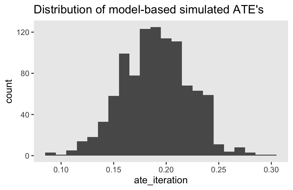
# summarize across the iterations
sim %>% 
  summarise(mean = mean(ate_iteration),
            sd = sd(ate_iteration))

## # A tibble: 1 × 2
##    mean     sd
##   <dbl>  <dbl>
## 1 0.192 0.0321

The mean¹¹ of our random process is a pretty good approximation of our estimate for \(\tau_\text{ATE}\) computed from the avg_comparisons() function, above.

Backing up a bit, we might want to get a better sense of all those \(\hat p_i^1\), \(\hat p_i^0\), and \((\hat p_i^1 - \hat p_i^0)\) estimates we’ve been averaging over. Like in the last post, we’ll display them in a couple coefficient plots. To keep down the clutter, we’ll restrict ourselves to a random \(n = 50\) subset of the 400 cases in the wilson2017 data.

# define the random subset
set.seed(3)

id_subset <- wilson2017 %>%
  slice_sample(n = 50) %>% 
  pull(id)

# counterfactual probabilities
p1 <- predictions(glm1, newdata = nd) %>% 
  data.frame() %>% 
  filter(id %in% id_subset) %>% 
  mutate(y = ifelse(tx == 0, "hat(italic(p))^0", "hat(italic(p))^1")) %>% 
  
  ggplot(aes(x = estimate, y = reorder(id, estimate), color = y)) +
  geom_interval(aes(xmin = conf.low, xmax = conf.high),
                position = position_dodge(width = -0.2),
                size = 1/5) +
  geom_point(aes(shape = y),
             size = 2) +
  scale_color_viridis_d(NULL, option = "A", begin = .3, end = .6,
                        labels = scales::parse_format()) +
  scale_shape_manual(NULL, values = c(20, 18),
                     labels = scales::parse_format()) +
  scale_x_continuous(limits = 0:1) +
  scale_y_discrete(breaks = NULL) +
  labs(subtitle = "Counterfactual probabilities",
       x = expression(hat(italic(p))[italic(i)]),
       y = "id (ranked)") +
  theme(legend.background = element_blank(),
        legend.position = c(.9, .85))

# treatment effects
p2 <- comparisons(glm1, newdata = nd, variables = "tx", by = "id") %>% 
  data.frame() %>% 
  filter(id %in% id_subset) %>% 
  
  ggplot(aes(x = estimate, y = reorder(id, estimate))) +
  geom_vline(xintercept = 0, color = "white") +
  geom_interval(aes(xmin = conf.low, xmax = conf.high),
                size = 1/5) +
  geom_point() +
  scale_x_continuous(limits = c(-0.5, 0.5)) +
  scale_y_discrete(breaks = NULL) +
  labs(subtitle = "Contrasts",
       x = expression(hat(italic(p))[italic(i)]^1-hat(italic(p))[italic(i)]^0),
       y = NULL) +
  theme(legend.background = element_blank(),
        legend.position = c(.9, .85))

# combine the two plots
p1 + p2 + plot_annotation(title = "Person-level estimates based on the logistic regression ANOVA model (glm1)")

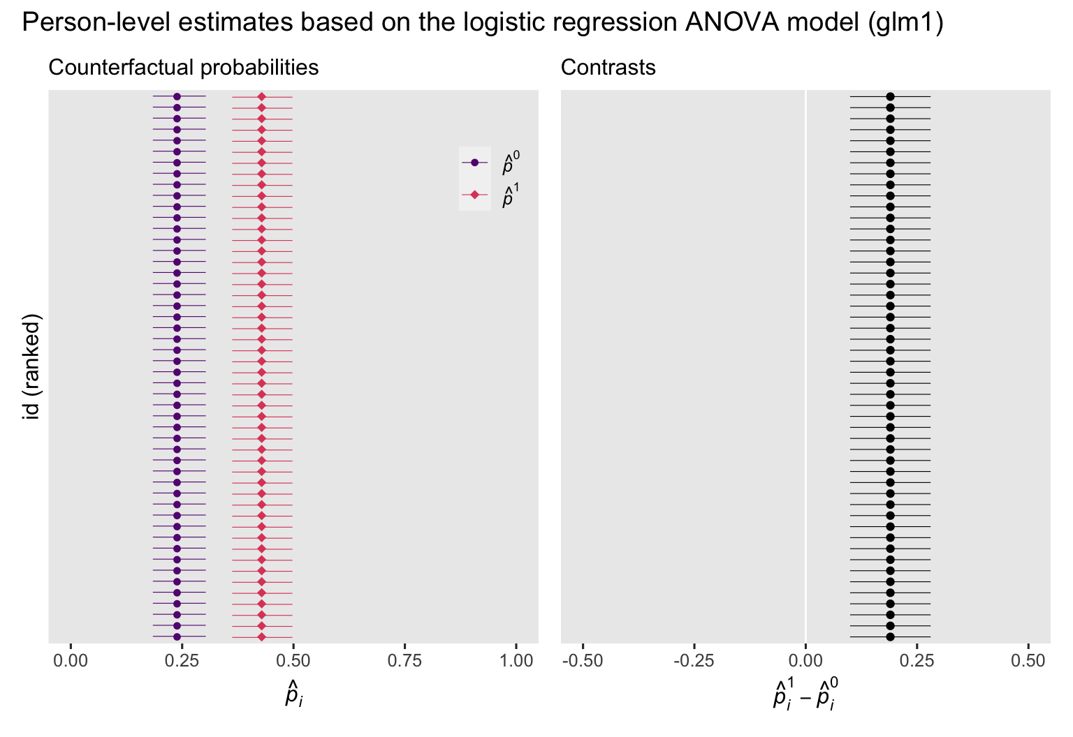
If the left plot, we see the counterfactual probabilities, depicted by their point estimates (dots) and 95% intervals (horizontal lines), and colored by whether they were based on the control condition \((\hat p_i^0)\) or the experimental intervention \((\hat p_i^1)\). In the right plot, we have the corresponding contrasts \((\hat p_i^1 - \hat p_i^0)\). In both plots, the y-axis has been rank ordered by the magnitudes of the estimates. Other than how we have switched from predictions \(\hat y_i\) to probabilities \(\hat p_i\), the overall results of these plots follow the same patterns as those in their analogues from the last post, where we used the conventional OLS framework. Because the logistic regression ANOVA model glm1 has no covariates, the probabilities and their contrasts are identical for all participants. As we’ll see later on, this will change when we switch to the ANCOVA model.

Another fine point that’s easy to lose track of is all those \((\hat p_i^1 - \hat p_i^0)\) contrasts in the right plot are NOT estimates for individual causal effects \((\tau_i)\). For binary data, individual causal effects can only take on values of \(-1\), \(0\), or \(1\). Even when we use the so-called standardization or g-computation method, our logistic regression models don’t really return individual treatment effects, even in the counterfactual sense. Rather, they return individual probability contrasts. But importantly, the average of those probability contrasts does return a valid estimate of the ATE. Wild, huh?

Wrapping up, in the case of an ANOVA-type logistic regression model of a randomized experiment,

• \(\operatorname{logit}^{-1}(\beta_0 + \beta_1) - \operatorname{logit}^{-1}(\beta_1)\),
• \(p^1 - p^0\), and
• \(\mathbb E (p_i^1 - p_i^0)\)

are all the same thing. They’re all equal to our primary estimand \(\tau_\text{ATE}\), the average treatment effect.

ATE for the ANCOVA

Now we’re ready to see how we might use our baseline covariates to better estimate the ATE from our logistic-regression ANCOVA. In our last post, we focused on a case where the only covariate was continuous. In this blog post, we’re analyzing a data set containing a mixture of continuous and discrete covariates. So for notation sake, let \(\mathbf C_i\) stand a vector of continuous covariates and let \(\mathbf D_i\) stand a vector of discrete covariates, both of which vary across the \(i\) cases. We can use these to help estimate the ATE with the formula:

$$\tau_\text{ATE} = \mathbb E (y_i^1 - y_i^0 \mid \mathbf C_i, \mathbf D_i).$$

In words, this means the average treatment effect in the population is the same as the average of each participant’s individual treatment effect, computed conditional on their continuous covariates \(\mathbf C_i\) and discrete covariates \(\mathbf D_i\). This, again, is sometimes called standardization or g-computation.¹² Within the context of a logistic regression model, we further observe

$$ \tau_\text{ATE} = \mathbb E (y_i^1 - y_i^0 \mid \mathbf C_i, \mathbf D_i) = {\color{blueviolet}{\mathbb E (p_i^1 - p_i^0 \mid \mathbf C_i, \mathbf D_i)}}, $$

where \(p_i^1\) and \(p_i^0\) are the counterfactual probabilities for each of the \(i\) cases, estimated in light of their covariate values.

Whether we have continuous covariates, discrete covariates, or a combination of both, the standardization method works the same. However, this is no longer the case when using the difference in population means approach, the covariate-adjusted version of \(\mathbb E (y_i^1) - \mathbb E (y_i^0)\). One complication is we might not be able to mean-center the discrete covariates in our \(\mathbf D\) vector. Sometimes people will mean center dummy variables, which can lead to awkward interpretive issues.¹³ But even this approach will not generalize well to multi-categorical nominal variables, like ethnicity. Another solution is to set discrete covariates at their modes (see Muller & MacLehose, 2014), which we’ll denote \(\mathbf D^m\). This gives us a new estimand:

$$\tau_\text{TEMM} = \operatorname{\mathbb{E}} \left (y_i^1 \mid \mathbf{\bar C}, \mathbf D^m \right) - \operatorname{\mathbb{E}} \left (y_i^0 \mid \mathbf{\bar C}, \mathbf D^m \right),$$

where TEMM is an acronym for treatment effect at the mean and/or mode. We’ll see what this looks like for our wilson2017 data in a bit. In the meantime, beware the TEMM acronym is not widely used in the literature; I’m just using it here to help clarify a point. More importantly, once you move beyond the ATE to specify particular values for \(\mathbf C\) and/or \(\mathbf D\), you’re really just computing one form or another of the conditional average treatment effect (CATE; \(\tau_\text{CATE}\)), which we might clarify with the formula

$$\tau_\text{CATE} = \operatorname{\mathbb{E}}(y_i^1 \mid \mathbf C = \mathbf c, \mathbf D = \mathbf d) - \operatorname{\mathbb{E}}(y_i^0 \mid \mathbf C = \mathbf c, \mathbf D = \mathbf d),$$

where \(\mathbf C = \mathbf c\) is meant to convey you have chosen particular values \(\mathbf c\) for the variables in the \(\mathbf C\) vector, and \(\mathbf D = \mathbf d\) is meant to convey you have chosen particular values \(\mathbf d\) for the variables in the \(\mathbf D\) vector. In addition to means or modes, these values could be any which are of particular interest to researchers and their audiences.

Within the context of a logistic regression model, we further observe

$$ \begin{align*} \tau_\text{TEMM} & = \operatorname{\mathbb{E}} \left (y_i^1 \mid \mathbf{\bar C}, \mathbf D^m \right) - \operatorname{\mathbb{E}} \left (y_i^0 \mid \mathbf{\bar C}, \mathbf D^m \right) \\ & = {\color{blueviolet}{\left (p^1 \mid \mathbf{\bar C}, \mathbf D^m \right) - \left (p^0 \mid \mathbf{\bar C}, \mathbf D^m \right)}} \end{align*} $$

where \(p_i^1\) and \(p_i^0\) are the counterfactual probabilities for each of the \(i\) cases, estimated in light of their covariate values. In a similar way

$$ \begin{align*} \tau_\text{CATE} & = \operatorname{\mathbb{E}} (y_i^1 \mid \mathbf C = \mathbf c, \mathbf D = \mathbf d) - \operatorname{\mathbb{E}}(y_i^0 \mid \mathbf C = \mathbf c, \mathbf D = \mathbf d) \\ & = {\color{blueviolet}{(p^1 \mid \mathbf C = \mathbf c, \mathbf D = \mathbf d) - (p^0 \mid \mathbf C = \mathbf c, \mathbf D = \mathbf d)}}. \end{align*} $$

Importantly, we have some inequalities to consider:

$$ \begin{align*} \mathbb E (y_i^1 - y_i^0 \mid \mathbf C_i, \mathbf D_i) & \neq \operatorname{\mathbb{E}} \left (y_i^1 \mid \mathbf{\bar C}, \mathbf D^m \right) - \operatorname{\mathbb{E}} \left (y_i^0 \mid \mathbf{\bar C}, \mathbf D^m \right) \\ & \neq \operatorname{\mathbb{E}} (y_i^1 \mid \mathbf C = \mathbf c, \mathbf D = \mathbf d) - \operatorname{\mathbb{E}} (y_i^0 \mid \mathbf C = \mathbf c, \mathbf D = \mathbf d) \end{align*} $$

and thus

$$ \begin{align*} \mathbb E (p_i^1 - p_i^0 \mid \mathbf C_i, \mathbf D_i) & \neq \left (p^1 \mid \mathbf{\bar C}, \mathbf D^m \right) - \left (p^0 \mid \mathbf{\bar C}, \mathbf D^m \right) \\ & \neq (p^1 \mid \mathbf C = \mathbf c, \mathbf D = \mathbf d) - (p^0 \mid \mathbf C = \mathbf c, \mathbf D = \mathbf d), \end{align*} $$

which means

$$ \begin{align*} \tau_\text{ATE} & \neq \tau_\text{TEMM} \\ & \neq \tau_\text{CATE}. \end{align*} $$

This holds for logistic regression models regardless of whether you have discrete covariates. But enough with theory. Let’s bring this all to life with some application.

\(\beta_1\) in the logistic regression ANCOVA.

Earlier we learned the coefficient for the experimental group, \(\beta_1\), does not have a direct relation with the ATE for the logistic regression ANOVA model. In a similar way, the \(\beta_1\) coefficient does not have a direct relation with the ATE for the logistic regression ANCOVA model, either. If you want the ATE, you’ll have to use the methods from the sections to come. In the meantime, let’s compare the \(\beta_1\) estimates for the ANOVA and ANCOVA models.

bind_rows(tidy(glm1), tidy(glm2)) %>% 
  filter(term == "tx") %>% 
  mutate(fit = c("glm1", "glm2"),
         model_type = c("ANOVA", "ANCOVA")) %>%
  rename(`beta[1]` = estimate) %>% 
  select(fit, model_type, `beta[1]`, std.error)

## # A tibble: 2 × 4
##   fit   model_type `beta[1]` std.error
##   <chr> <chr>          <dbl>     <dbl>
## 1 glm1  ANOVA          0.873     0.219
## 2 glm2  ANCOVA         1.05      0.239

Unlike what typically occurs with OLS-based models, the standard error for \(\beta_1\) increased when we added the baseline covariates to the model. It turns out this will generally happen with logistic regression models, even when using high-quality covariates ( Robinson & Jewell, 1991; see also Ford & Norrie, 2002). This does not, however, mean we should not use baseline covariates in our logistic regression models. Rather, it means that we need to focus on how to compute the ATE, rather than fixate on the model coefficients (cf. Daniel et al., 2021). This can be very unsettling for those with strong roots in the OLS framework–it was for me. All I can say is: Your OLS sensibilities will not help you, here. The sooner you shed them, the better.

Compute \(\left (p^1 \mid \mathbf{\bar C}, \mathbf D^m \right) - \left (p^0 \mid \mathbf{\bar C}, \mathbf D^m \right)\) from glm2.

With our ANCOVA-type glm2 model, we can compute \(\left (p^1 \mid \mathbf{\bar C}, \mathbf D^m \right)\) and \(\left (p^0 \mid \mathbf{\bar C}, \mathbf D^m \right)\) with the base R predict() function. As a first step, we’ll define our prediction grid with the sample mean for our continuous covariate agez, the sample modes for our four discrete covariates, and then expand the grid to include both values of the experimental dummy. This presents a small difficulty, however, because base R does not have a function for modes. Here we’ll make one ourselves.

get_mode <- function(x) {
  ux <- unique(x)
  ux[which.max(tabulate(match(x, ux)))]
}

This get_mode() function is used internally by the marginaleffects package (see here), and has its origins in this stackoverflow discussion. Here’s how we can use get_mode() to help us make the nd data grid.

nd <- wilson2017 %>% 
  summarise(agez      = 0,  # recall agez is a z-score, with a mean of 0 by definition
            gender    = get_mode(gender),
            msm       = get_mode(msm),
            ethnicgrp = get_mode(ethnicgrp),
            partners  = get_mode(partners)) %>% 
  expand_grid(tx = 0:1)

# what is this?
print(nd)

## # A tibble: 2 × 6
##    agez gender msm   ethnicgrp            partners    tx
##   <dbl> <fct>  <fct> <fct>                <fct>    <int>
## 1     0 Female other White/ White British 1            0
## 2     0 Female other White/ White British 1            1

Thus we will be computing our estimate for \(\tau_\text{TEMM}\) based on a White 23-year-old woman who had one sexual partner over the past year. By definition, such a person would not be a man who has sex with men (msm == 1). Also, we know this person is 23 years old because agez == 0 at that value. Here’s the proof.

wilson2017 %>% 
  summarise(mean_age = mean(age))

## # A tibble: 1 × 1
##   mean_age
##      <dbl>
## 1     22.9

Now we pump these values into predict().

predict(glm2, 
        newdata = nd,
        se.fit = TRUE,
        type = "response") %>% 
  data.frame() %>% 
  bind_cols(nd)

##         fit     se.fit residual.scale agez gender   msm            ethnicgrp partners tx
## 1 0.2056724 0.04762467              1    0 Female other White/ White British        1  0
## 2 0.4263581 0.06109031              1    0 Female other White/ White British        1  1

To get the contrast with standard errors and so on, we switch to the predictions() function and set hypothesis = "revpairwise".

# conditional probabilities
predictions(glm2, newdata = nd, by = "tx")

## 
##  tx Estimate Pr(>|z|) 2.5 % 97.5 % agez gender   msm            ethnicgrp partners
##   0    0.206   <0.001 0.128  0.314    0 Female other White/ White British        1
##   1    0.426    0.235 0.313  0.548    0 Female other White/ White British        1
## 
## Columns: rowid, tx, estimate, p.value, conf.low, conf.high, agez, gender, msm, ethnicgrp, partners, anytest

# TEMM
predictions(glm2, newdata = nd, by = "tx", hypothesis = "revpairwise")

## 
##   Term Estimate Std. Error    z Pr(>|z|) 2.5 % 97.5 %
##  1 - 0    0.221     0.0488 4.52   <0.001 0.125  0.316
## 
## Columns: term, estimate, std.error, statistic, p.value, conf.low, conf.high

Thus we expect our hypothetical participant with demographics at the mean and/or modes for the covariates will be about 22% more likely to get tested if given the intervention, compared to if she had not.

Compute \((p^1 \mid \mathbf C = \mathbf c, \mathbf D = \mathbf d) - (p^0 \mid \mathbf C = \mathbf c, \mathbf D = \mathbf d)\) from glm2.

Since the \(\tau_\text{TEMM}\) is just a special case of a \(\tau_\text{CATE}\), we might practice computing an estimate for \(\tau_\text{CATE}\) with a different set of covariate values. Men who have sex with men (MSM) were one of the vulnerable subgroups of interest in Wilson et al. ( 2017), so we might take a look to see which combination of covariate values was most common for MSM in our subset of the data.

wilson2017 %>% 
  filter(msm == "msm") %>% 
  count(age, agez, ethnicgrp, partners) %>% 
  arrange(desc(n))

## # A tibble: 45 × 5
##      age    agez ethnicgrp            partners     n
##    <dbl>   <dbl> <fct>                <fct>    <int>
##  1    26  0.894  White/ White British 10+          5
##  2    28  1.46   White/ White British 10+          4
##  3    24  0.323  White/ White British 10+          3
##  4    21 -0.533  White/ White British 10+          2
##  5    23  0.0378 White/ White British 5            2
##  6    25  0.609  White/ White British 6            2
##  7    26  0.894  White/ White British 6            2
##  8    29  1.75   White/ White British 5            2
##  9    18 -1.39   White/ White British 5            1
## 10    19 -1.10   White/ White British 4            1
## # ℹ 35 more rows

It appears we’re now interested in computing \(\tau_\text{CATE}\) for a White 26-year-old MSM who had 10 or more partners over the past year. Let’s redefine our nd predictor grid accordingly.

nd <- wilson2017 %>% 
  filter(msm == "msm") %>% 
  count(age, agez, gender, msm, ethnicgrp, partners) %>% 
  arrange(desc(n)) %>% 
  slice(1) %>% 
  select(-n) %>% 
  expand_grid(tx = 0:1)

# what now?
print(nd)

## # A tibble: 2 × 7
##     age  agez gender msm   ethnicgrp            partners    tx
##   <dbl> <dbl> <fct>  <fct> <fct>                <fct>    <int>
## 1    26 0.894 Male   msm   White/ White British 10+          0
## 2    26 0.894 Male   msm   White/ White British 10+          1

Now use the predictions() function to estimate the desired counterfactual probabilities and the estimate for this version of \(\tau_\text{CATE}\).

# conditional probabilities
predictions(glm2, newdata = nd, by = "tx")

## 
##  tx Estimate Pr(>|z|) 2.5 % 97.5 % age  agez gender msm            ethnicgrp partners
##   0    0.259  0.00919 0.137  0.435  26 0.894   Male msm White/ White British      10+
##   1    0.501  0.99481 0.306  0.695  26 0.894   Male msm White/ White British      10+
## 
## Columns: rowid, tx, estimate, p.value, conf.low, conf.high, age, agez, gender, msm, ethnicgrp, partners, anytest

# CATE
predictions(glm2, newdata = nd, by = "tx", hypothesis = "revpairwise")

## 
##   Term Estimate Std. Error   z Pr(>|z|) 2.5 % 97.5 %
##  1 - 0    0.242     0.0589 4.1   <0.001 0.126  0.357
## 
## Columns: term, estimate, std.error, statistic, p.value, conf.low, conf.high

Turns out our estimate for this \(\tau_\text{CATE}\) is a little larger than our estimate for \(\tau_\text{TEMM}\), from above. With this framework, you can compute \(\tau_\text{CATE}\) estimates for any number of theoretically-meaningful covariate sets.

Compute \(\mathbb E (p_i^1 - p_i^0 \mid \mathbf C_i, \mathbf D_i)\) from glm2.

Before we compute our counterfactual \(\mathbb{E}(\hat p_i^1 - \hat p_i^0 \mid \mathbf C_i, \mathbf D_i)\) estimates from our ANCOVA-type logistic regression model glm2, we’ll first need to redefine our nd predictor data. This time, we’ll retain the full set of covariate values for each participant.

nd <- wilson2017 %>% 
  select(id, age, agez, gender, msm, ethnicgrp, partners) %>% 
  expand_grid(tx = 0:1)

# what?
glimpse(nd)

## Rows: 800
## Columns: 8
## $ id        <dbl> 20766, 20766, 18778, 18778, 15678, 15678, 20253, 20253, 23805, 23805, 17549, 17549, 16627,…
## $ age       <dbl> 21, 21, 19, 19, 17, 17, 20, 20, 24, 24, 19, 19, 18, 18, 20, 20, 29, 29, 28, 28, 20, 20, 23…
## $ agez      <dbl> -0.53290527, -0.53290527, -1.10362042, -1.10362042, -1.67433557, -1.67433557, -0.81826284,…
## $ gender    <fct> Male, Male, Male, Male, Female, Female, Male, Male, Female, Female, Female, Female, Male, …
## $ msm       <fct> other, other, other, other, other, other, other, other, other, other, other, other, other,…
## $ ethnicgrp <fct> White/ White British, White/ White British, White/ White British, White/ White British, Mi…
## $ partners  <fct> 2, 2, 4, 4, 2, 2, 1, 1, 4, 4, 2, 2, 1, 1, 2, 2, 10+, 10+, 1, 1, 1, 1, 1, 1, 1, 1, 1, 1, 2,…
## $ tx        <int> 0, 1, 0, 1, 0, 1, 0, 1, 0, 1, 0, 1, 0, 1, 0, 1, 0, 1, 0, 1, 0, 1, 0, 1, 0, 1, 0, 1, 0, 1, …

Instead of first practicing computing the probabilities with base R predict(), let’s just jump directly to the precitions() and comparisons() functions from the marginaleffects package.

# here are the counterfactual probabilities
predictions(glm2, newdata = nd) %>% 
  head(n = 10)

## 
##  Estimate Pr(>|z|)  2.5 % 97.5 %    id age   agez gender   msm                 ethnicgrp partners tx
##    0.1202  < 0.001 0.0553  0.242 20766  21 -0.533 Male   other White/ White British             2  0
##    0.2816  0.02200 0.1496  0.466 20766  21 -0.533 Male   other White/ White British             2  1
##    0.0812  < 0.001 0.0319  0.192 18778  19 -1.104 Male   other White/ White British             4  0
##    0.2023  0.00317 0.0925  0.387 18778  19 -1.104 Male   other White/ White British             4  1
##    0.1068  < 0.001 0.0414  0.249 15678  17 -1.674 Female other Mixed/ Multiple ethnicity        2  0
##    0.2555  0.03380 0.1134  0.480 15678  17 -1.674 Female other Mixed/ Multiple ethnicity        2  1
##    0.0938  < 0.001 0.0455  0.184 20253  20 -0.818 Male   other White/ White British             1  0
##    0.2291  < 0.001 0.1303  0.371 20253  20 -0.818 Male   other White/ White British             1  1
##    0.2019  0.00122 0.0991  0.368 23805  24  0.323 Female other White/ White British             4  0
##    0.4207  0.42048 0.2501  0.613 23805  24  0.323 Female other White/ White British             4  1
## 
## Columns: rowid, estimate, p.value, conf.low, conf.high, id, age, agez, gender, msm, ethnicgrp, partners, tx, anytest

# here are the contrasts based on those probabilities
comparisons(glm2, newdata = nd, variables = "tx") %>% 
  head(n = 10)

## 
##  Term Contrast Estimate Std. Error    z Pr(>|z|)  2.5 % 97.5 %    id age   agez gender   msm
##    tx    1 - 0    0.161     0.0507 3.18  0.00145 0.0621  0.261 20766  21 -0.533 Male   other
##    tx    1 - 0    0.161     0.0507 3.18  0.00145 0.0621  0.261 20766  21 -0.533 Male   other
##    tx    1 - 0    0.121     0.0455 2.66  0.00784 0.0318  0.210 18778  19 -1.104 Male   other
##    tx    1 - 0    0.121     0.0455 2.66  0.00784 0.0318  0.210 18778  19 -1.104 Male   other
##    tx    1 - 0    0.149     0.0563 2.64  0.00824 0.0384  0.259 15678  17 -1.674 Female other
##    tx    1 - 0    0.149     0.0563 2.64  0.00824 0.0384  0.259 15678  17 -1.674 Female other
##    tx    1 - 0    0.135     0.0401 3.37  < 0.001 0.0567  0.214 20253  20 -0.818 Male   other
##    tx    1 - 0    0.135     0.0401 3.37  < 0.001 0.0567  0.214 20253  20 -0.818 Male   other
##    tx    1 - 0    0.219     0.0548 3.99  < 0.001 0.1113  0.326 23805  24  0.323 Female other
##    tx    1 - 0    0.219     0.0548 3.99  < 0.001 0.1113  0.326 23805  24  0.323 Female other
##                  ethnicgrp partners
##  White/ White British             2
##  White/ White British             2
##  White/ White British             4
##  White/ White British             4
##  Mixed/ Multiple ethnicity        2
##  Mixed/ Multiple ethnicity        2
##  White/ White British             1
##  White/ White British             1
##  White/ White British             4
##  White/ White British             4
## 
## Columns: rowid, term, contrast, estimate, std.error, statistic, p.value, conf.low, conf.high, predicted, predicted_hi, predicted_lo, id, age, agez, gender, msm, ethnicgrp, partners, tx, anytest

Even among the first 10 rows, we can see there’s a lot of diversity among the estimates for the individual probability contrasts. Before we compute the ATE, it might be worth the effort to look more closely at the participant-level estimates in a coefficient plot. As with the ANOVA model, we’ll only visualize an \(n = 50\) subset of the 400 cases.

# counterfactual probabilities
p3 <- predictions(glm2, newdata = nd) %>% 
  data.frame() %>% 
  filter(id %in% id_subset) %>% 
  mutate(y = ifelse(tx == 0, "hat(italic(p))^0", "hat(italic(p))^1")) %>% 
  
  ggplot(aes(x = estimate, y = reorder(id, estimate), color = y)) +
  geom_interval(aes(xmin = conf.low, xmax = conf.high),
                position = position_dodge(width = -0.2),
                size = 1/5) +
  geom_point(aes(shape = y),
             size = 2) +
  scale_color_viridis_d(NULL, option = "A", begin = .3, end = .6,
                        labels = scales::parse_format()) +
  scale_shape_manual(NULL, values = c(20, 18),
                     labels = scales::parse_format()) +
  scale_x_continuous(limits = 0:1) +
  scale_y_discrete(breaks = NULL) +
  labs(subtitle = "Counterfactual probabilities",
       x = expression(hat(italic(p))[italic(i)]),
       y = "id (ranked)") +
  theme(legend.background = element_blank(),
        legend.position = c(.9, .85))

# treatment effects
p4 <- comparisons(glm2, newdata = nd, variables = "tx") %>% 
  data.frame() %>% 
  filter(id %in% id_subset) %>% 
  
  ggplot(aes(x = estimate, y = reorder(id, estimate))) +
  geom_vline(xintercept = 0, color = "white") +
  geom_interval(aes(xmin = conf.low, xmax = conf.high),
                size = 1/5) +
  geom_point() +
  scale_x_continuous(limits = c(-0.5, 0.5)) +
  scale_y_discrete(breaks = NULL) +
  labs(subtitle = "Contrasts",
       x = expression(hat(italic(p))[italic(i)]^1-hat(italic(p))[italic(i)]^0),
       y = NULL) +
  theme(legend.background = element_blank(),
        legend.position = c(.9, .85))

# combine
p3 + p4 + plot_annotation(title = "Person-level estimates based on the logistic regression ANCOVA model (glm2)")

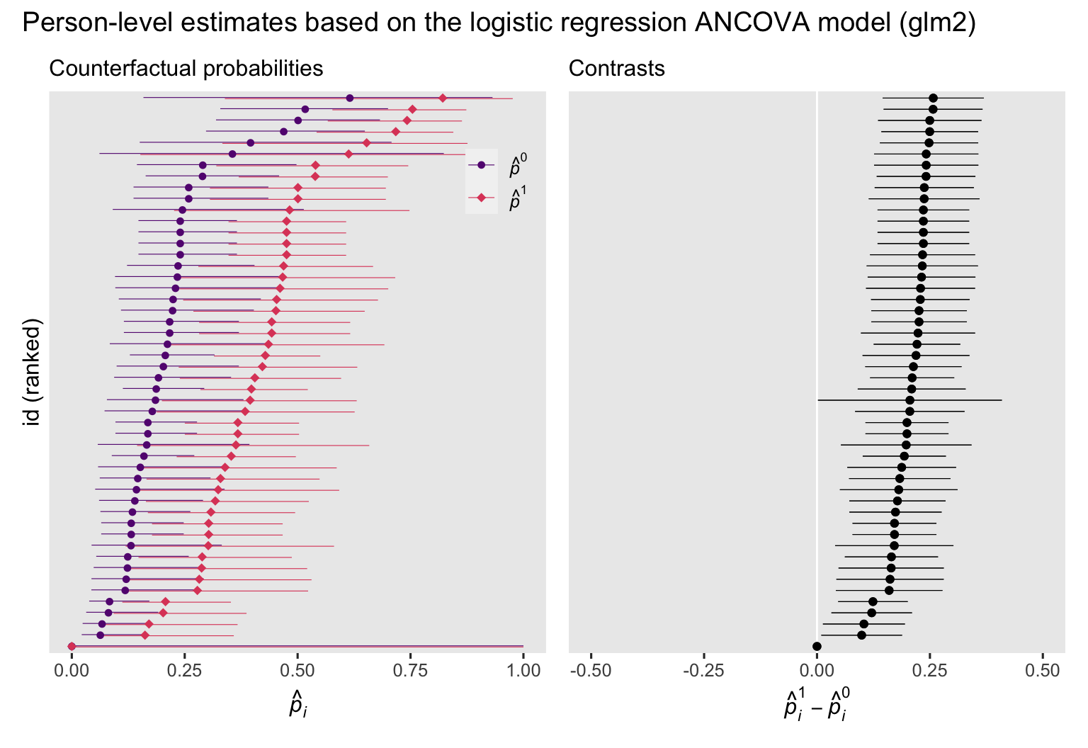
Now we have added covariates to the model, the counterfactual probabilities vary across participants, which was the same pattern for the OLS-based ANCOVA from the last post, too. But unlike with the ANOVA model and unlike with the ANCOVA results from the last post, the \((p_i^1 - p_i^0)\) contrasts now vary across participants. Once you leave the simple OLS paradigm, this issue will come up again and again when you fit ANCOVA models. Covariate values often change the magnitudes of the probability estimates and their contrasts.

Investigating further, here’s the full distribution of the contrast values for all \(n = 400\) cases. To reduce visual complexity, we’ll drop the 95% confidence interval lines.

comparisons(glm2, newdata = nd, variables = "tx", by = "id") %>% 
  data.frame() %>% 
  
  ggplot(aes(x = estimate)) +
  geom_vline(xintercept = 0, color = "white") +
  geom_dots(layout = "swarm", color = "gray30", fill = "gray30") +
  stat_pointinterval(aes(y = -0.017), 
                     point_interval = mean_qi, .width = .5, 
                     point_size = 2.5, color = "red") +
  scale_x_continuous(limits = c(-0.5, 0.5)) +
  scale_y_continuous(NULL, breaks = NULL) +
  labs(title = "The individual contrast distribution",
       subtitle = "Each gray dot is a point estmiate for a single participant's\ncontrast. The horizontal red line marks off the interquartile\nrange, and the red dot marks the ATE.",
       x = expression(hat(italic(p))[italic(i)]^1-hat(italic(p))[italic(i)]^0)) +
  coord_cartesian(ylim = c(0, 0.7))

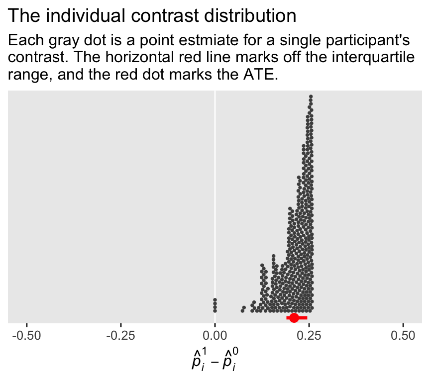
The red dot below the distribution marks off the average of the participant-level probability contrast estimates, which is the same as the point estimate for the ATE. Speaking of which, here’s our estimate of \(\tau_\text{ATE}\) for this model, and for the simpler ANOVA-type glm1.

bind_rows(
  avg_comparisons(glm1, newdata = nd, variables = "tx"),
  avg_comparisons(glm2, newdata = nd, variables = "tx")
) %>% 
  data.frame() %>% 
  mutate(fit = c("glm1", "glm2"),
         model_type = c("ANOVA", "ANCOVA")) %>%
  rename(`tau[ATE]` = estimate) %>% 
  select(fit, model_type, `tau[ATE]`, std.error)

##    fit model_type  tau[ATE]  std.error
## 1 glm1      ANOVA 0.1899927 0.04613649
## 2 glm2     ANCOVA 0.2102164 0.04502833

Whereas the standard error for the \(\beta_1\) coefficient increased when we added the baseline covariates to the model, the standard error for our primary estimand \(\tau_\text{ATE}\) decreased. This isn’t a fluke of our \(n = 400\) subset. The same general pattern holds for the full data set. Not only is \(\beta_1\) not the same as the ATE for a logistic regression model, adding covariates can have the reverse effect on their respective standard errors. This phenomena is related to the so-called noncollapsibility issue, which is well known among statisticians who work with medical trials. For an entry point into that literature, see Daniel et al. ( 2021) or Morris et al. ( 2022). If you prefer your statistics explained with sass, I find Jake Westfall’s ( 2018) blog post, Logistic regression is not fucked, an excellent and accessible introduction to the noncollapsibility issue. But anyway, yes, baseline covariates can help increase the precision with which you estimate the ATE from a logistic regression model. Don’t worry about what happens with \(\beta_1\). Focus on the ATE.

Grappling with \((p_i^1 - p_i^0 \mid \mathbf C_i, \mathbf D_i)\) distributions.

Given how the logistic-regression-based participant-level probability contrasts now come in distributions when estimated from ANCOVA models, some researchers have wondered whether it’s a good idea to use a single summary value like the ATE. Biostatistician Frank Harrell, for example, recommended displaying the entire contrast distribution in his ( 2021) blog post, Avoiding one-number summaries of treatment effects for RCTs with binary outcomes. Albuquerque and Arel-Bundock covered Harrell’s primary material from a marginaleffects perspective in their ( 2023) vignette, Logistic regression (see also Kent & Hayward, 2007). At the moment, I’m still inclined to rely on the ATE, but perhaps also show a plot of the contrast distribution as a supplement.

Another approach might be to focus on one or a handful of CATE’s. This, however, I would only recommend with great caution. To help clarify why, let’s compute the CATE for every valid combination of our baseline covariate values. First, we’ll update our nd data grid.

nd <- crossing(
  agez      = distinct(wilson2017, agez) %>% pull(),
  gender    = distinct(wilson2017, gender) %>% pull(),
  msm       = distinct(wilson2017, msm) %>% pull(),
  ethnicgrp = distinct(wilson2017, ethnicgrp) %>% pull(),
  partners  = distinct(wilson2017, partners) %>% pull()) %>% 
  # remove the impossible cases of Females who are also MSM
  filter((gender == "Female" & msm == "other") | gender == "Male") %>% 
  # throw in an id index
  mutate(id = 1:n()) %>% 
  expand_grid(tx = 0:1)

# what?
glimpse(nd)

## Rows: 4,500
## Columns: 7
## $ agez      <dbl> -1.959693, -1.959693, -1.959693, -1.959693, -1.959693, -1.959693, -1.959693, -1.959693, -1…
## $ gender    <fct> Female, Female, Female, Female, Female, Female, Female, Female, Female, Female, Female, Fe…
## $ msm       <fct> other, other, other, other, other, other, other, other, other, other, other, other, other,…
## $ ethnicgrp <fct> White/ White British, White/ White British, White/ White British, White/ White British, Wh…
## $ partners  <fct> 1, 1, 2, 2, 3, 3, 4, 4, 5, 5, 6, 6, 7, 7, 8, 8, 9, 9, 10+, 10+, 1, 1, 2, 2, 3, 3, 4, 4, 5,…
## $ id        <int> 1, 1, 2, 2, 3, 3, 4, 4, 5, 5, 6, 6, 7, 7, 8, 8, 9, 9, 10, 10, 11, 11, 12, 12, 13, 13, 14, …
## $ tx        <int> 0, 1, 0, 1, 0, 1, 0, 1, 0, 1, 0, 1, 0, 1, 0, 1, 0, 1, 0, 1, 0, 1, 0, 1, 0, 1, 0, 1, 0, 1, …

Now we’ll summarize the results with a plot of the point estimates (left), and a plot their standard errors (right).

# compute/save the point estimate and standard error for the ATE
ate_est <- avg_comparisons(glm2, variables = "tx") %>% pull(estimate)
ate_se <- avg_comparisons(glm2, variables = "tx") %>% pull(std.error)

# point estimates
p5 <- comparisons(glm2, newdata = nd, variables = "tx", by = "id")  %>% 
  data.frame() %>% 
  
  ggplot(aes(x = estimate)) +
  geom_histogram(boundary = 0, binwidth = 0.01) +
  geom_vline(xintercept = ate_est, color = "red") +
  scale_y_continuous(limits = c(0, 450)) +
  labs(subtitle = "The red line marks the ATE point estimate.",
       x = expression(widehat(CATE)))

# standard errors
p6 <- comparisons(glm2, newdata = nd, variables = "tx", by = "id")  %>% 
  data.frame() %>% 
  
  ggplot(aes(x = std.error)) +
  geom_histogram(boundary = 0, binwidth = 0.005) +
  geom_vline(xintercept = ate_se, color = "red") +
  scale_y_continuous(NULL, breaks = NULL, limits = c(0, 450)) +
  labs(subtitle = "The red line marks the ATE standard error.",
       x = expression(CATE[italic(SE)]))

# combine
p5 + p6 + 
  plot_annotation(title = "CATE distributions based on the logistic regression ANCOVA model (glm2)",
                  subtitle = "These plots are based on 2,250 possible combinations of covariate values.")

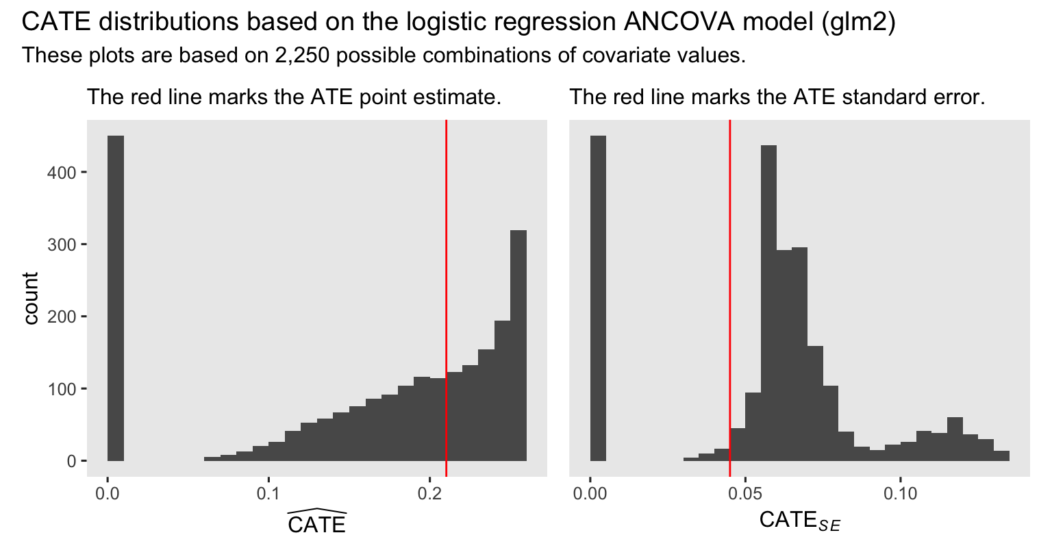
The ATE is still near the middle of the distribution of point estimates for the CATE’s. However, the standard error for the ATE is well lower than the bulk of the standard errors for the various versions of the CATE. If you have designed and powered a study to compute the ATE, be very cautious about switching your focus to the CATE. You might not have the right data set to do a good job estimating the CATE with precision.

In case you were wondering, all those counterfactual cases with near-zero point estimates and near-zero standard errors had Other as the value for ethnicgrp. If you look back up to the model summary for glm2, you’ll notice the coefficient for that category has a very low point estimate and an extremely large standard error. This is what can happen when you include a categorical variable with only a handful of cases for one of the categories in a frequentist logistic regression model. Happily, this will be a much smaller problem when we adopt a Bayesian framework in the next post.

Words are hard

Before we wrap up, y’all should beware the language of ATE is not uniformly used among researchers who use logistic regression for causal inference. For example, Gelman and colleagues used the language of “the difference in probabilities” on page 225 of their ( 2020) textbook. McCabe et al. ( 2022) used the language of discrete differences “to define a marginal effect as the difference between two points on a regression function” (p. 247), which is what we’re doing in the special case of a randomized experiment. Agresti & Tarantola ( 2018) used the term discrete change for discrete variables and average marginal effect for continuous ones. Mood ( 2010), differentiated discrete and continuous models by calling the ATE from a logistic regression model \(\Delta{P}\), and using the term average marginal effect when computing the ATE from a conventional Gaussian model.

Recap

In this post, some of the main points we covered were:

• With logistic regression, the \(\beta_1\) coefficient has no direct relationship with the ATE, regardless of whether you have included covariates.
• For the logistic regression ANOVA model,
  • \(\tau_\text{ATE} = \mathbb E (p_i^1 - p_i^0)\), and
  • \(\tau_\text{ATE} = p^1 - p^0\).
• For the logistic regression ANCOVA model,
  • \(\tau_\text{ATE} = \mathbb E (p_i^1 - p_i^0 \mid \mathbf C_i, \mathbf D_i)\), but
  • \(\tau_\text{CATE} = (p^1 \mid \mathbf C = \mathbf c, \mathbf D = \mathbf d) - (p^0 \mid \mathbf C = \mathbf c, \mathbf D = \mathbf d)\).
• For a logistic regression ANCOVA model, there can be many different values for the conditional average treatment effect, \(\tau_\text{CATE}\), depending which values one uses for the covariates.
• With logistic regression models, baseline covariates tend to
  • increase the standard errors for the \(\beta_1\) coefficient, and
  • decrease the standard errors for the average treatment effect, \(\tau_\text{ATE}\).

In the next post, we’ll explore how our causal inference methods work within an applied Bayesian statistics framework. We’ll practice with both simple Gaussian models, and logistic regression models, too. Until then, happy modeling, friends!

Thank a friend

I became aware of Wilson et al. ( 2017) through the follow-up paper by Morris et al. ( 2022). Morris and colleagues compared several ways to analyze these data, one of which was the standardization approach for logistic regression, such as we have done here. However, Morris and colleagues used a STATA-based workflow for their paper, and it was A. Jordan Nafa’s kind efforts (see here) which helped me understand how to use these methods in R.

Thank the reviewers

I’d like to publicly acknowledge and thank

• Isabella R. Ghement and
• Stephen J. Wild

for their kind efforts reviewing the draft of this post. Go team!

Do note the final editorial decisions were my own, and I do not think it would be reasonable to assume my reviewers have given blanket endorsements of the current version of this post.

Session information

sessionInfo()

## R version 4.3.0 (2023-04-21)
## Platform: aarch64-apple-darwin20 (64-bit)
## Running under: macOS Ventura 13.4
## 
## Matrix products: default
## BLAS:   /Library/Frameworks/R.framework/Versions/4.3-arm64/Resources/lib/libRblas.0.dylib 
## LAPACK: /Library/Frameworks/R.framework/Versions/4.3-arm64/Resources/lib/libRlapack.dylib;  LAPACK version 3.11.0
## 
## locale:
## [1] en_US.UTF-8/en_US.UTF-8/en_US.UTF-8/C/en_US.UTF-8/en_US.UTF-8
## 
## time zone: America/Chicago
## tzcode source: internal
## 
## attached base packages:
## [1] stats     graphics  grDevices utils     datasets  methods   base     
## 
## other attached packages:
##  [1] patchwork_1.1.2        ggdist_3.3.0           broom_1.0.5            flextable_0.9.1       
##  [5] marginaleffects_0.12.0 lubridate_1.9.2        forcats_1.0.0          stringr_1.5.0         
##  [9] dplyr_1.1.2            purrr_1.0.1            readr_2.1.4            tidyr_1.3.0           
## [13] tibble_3.2.1           ggplot2_3.4.2          tidyverse_2.0.0       
## 
## loaded via a namespace (and not attached):
##  [1] tidyselect_1.2.0        viridisLite_0.4.2       farver_2.1.1            fastmap_1.1.1          
##  [5] blogdown_1.17           fontquiver_0.2.1        promises_1.2.0.1        digest_0.6.31          
##  [9] timechange_0.2.0        mime_0.12               lifecycle_1.0.3         gfonts_0.2.0           
## [13] ellipsis_0.3.2          magrittr_2.0.3          compiler_4.3.0          rlang_1.1.1            
## [17] sass_0.4.6              tools_4.3.0             utf8_1.2.3              yaml_2.3.7             
## [21] data.table_1.14.8       knitr_1.43              labeling_0.4.2          askpass_1.1            
## [25] emo_0.0.0.9000          curl_5.0.1              xml2_1.3.4              httpcode_0.3.0         
## [29] withr_2.5.0             grid_4.3.0              fansi_1.0.4             gdtools_0.3.3          
## [33] xtable_1.8-4            colorspace_2.1-0        scales_1.2.1            MASS_7.3-58.4          
## [37] insight_0.19.2          crul_1.4.0              cli_3.6.1               rmarkdown_2.22         
## [41] crayon_1.5.2            ragg_1.2.5              generics_0.1.3          rstudioapi_0.14        
## [45] tzdb_0.4.0              readxl_1.4.2            katex_1.4.1             cachem_1.0.8           
## [49] assertthat_0.2.1        cellranger_1.1.0        vctrs_0.6.3             V8_4.3.0               
## [53] jsonlite_1.8.5          fontBitstreamVera_0.1.1 bookdown_0.34           hms_1.1.3              
## [57] beeswarm_0.4.0          systemfonts_1.0.4       xslt_1.4.4              jquerylib_0.1.4        
## [61] glue_1.6.2              equatags_0.2.0          distributional_0.3.2    stringi_1.7.12         
## [65] gtable_0.3.3            later_1.3.1             munsell_0.5.0           pillar_1.9.0           
## [69] htmltools_0.5.5         openssl_2.0.6           R6_2.5.1                textshaping_0.3.6      
## [73] evaluate_0.21           shiny_1.7.4             highr_0.10              backports_1.4.1        
## [77] fontLiberation_0.1.0    httpuv_1.6.11           bslib_0.5.0             Rcpp_1.0.10            
## [81] zip_2.3.0               uuid_1.1-0              checkmate_2.2.0         officer_0.6.2          
## [85] xfun_0.39               pkgconfig_2.0.3

References

Agresti, A., & Tarantola, C. (2018). Simple ways to interpret effects in modeling ordinal categorical data. Statistica Neerlandica, 72(3), 210–223. https://doi.org/10.1111/stan.12130
Albuquerque, A. M., & Arel-Bundock, V. (2023). Logistic regression. https://vincentarelbundock.github.io/marginaleffects/articles/logit.html
Arel-Bundock, V. (2023). Causal inference with the parametric g-formula. https://vincentarelbundock.github.io/marginaleffects/articles/gformula.html
Bartlett, J. W., Parra, C. O., & Daniel, R. M. (2023). G-formula for causal inference via multiple imputation. https://doi.org/10.48550/arXiv.2301.12026
Brumback, B. A. (2022). Fundamentals of causal inference with R. Chapman & Hall/CRC. https://www.routledge.com/Fundamentals-of-Causal-Inference-With-R/Brumback/p/book/9780367705053
Daniel, R., Zhang, J., & Farewell, D. (2021). Making apples from oranges: Comparing noncollapsible effect estimators and their standard errors after adjustment for different covariate sets. Biometrical Journal, 63(3), 528–557. https://doi.org/10.1002/bimj.201900297
Ford, I., & Norrie, J. (2002). The role of covariates in estimating treatment effects and risk in long-term clinical trials. Statistics in Medicine, 21(19), 2899–2908. https://doi.org/10.1002/sim.1294
Gelman, A., Hill, J., & Vehtari, A. (2020). Regression and other stories. Cambridge University Press. https://doi.org/10.1017/9781139161879
Harrell, F. (2021). Avoiding one-number summaries of treatment effects for RCTs with binary outcomes. https://www.fharrell.com/post/rdist/
Imbens, G. W., & Rubin, D. B. (2015). Causal inference in statistics, social, and biomedical sciences: An Introduction. Cambridge University Press. https://doi.org/10.1017/CBO9781139025751
Kent, D. M., & Hayward, R. A. (2007). Limitations of applying summary results of clinical trials to individual patients: The need for risk stratification. JAMA : The Journal of the American Medical Association, 298(10), 1209–1212. https://doi.org/10.1001/jama.298.10.1209
McCabe, C. J., Halvorson, M. A., King, K. M., Cao, X., & Kim, D. S. (2022). Interpreting interaction effects in generalized linear models of nonlinear probabilities and counts. Multivariate Behavioral Research, 57(2-3), 243–263. https://doi.org/10.1080/00273171.2020.1868966
Mood, C. (2010). Logistic regression: Why we cannot do what we think we can do, and what we can do about it. European Sociological Review, 26(1), 67–82. https://doi.org/10.1093/esr/jcp006
Morris, T. P., Walker, A. S., Williamson, E. J., & White, I. R. (2022). Planning a method for covariate adjustment in individually randomised trials: A practical guide. Trials, 23(1), 328. https://doi.org/10.1186/s13063-022-06097-z
Muller, C. J., & MacLehose, R. F. (2014). Estimating predicted probabilities from logistic regression: Different methods correspond to different target populations. International Journal of Epidemiology, 43(3), 962–970. https://doi.org/10.1093/ije/dyu029
Raab, G. M., Day, S., & Sales, J. (2000). How to select covariates to include in the analysis of a clinical trial. Controlled Clinical Trials, 21(4), 330–342. https://doi.org/10.1016/S0197-2456(00)00061-1
Robinson, L. D., & Jewell, N. P. (1991). Some surprising results about covariate adjustment in logistic regression models. International Statistical Review/Revue Internationale de Statistique, 227–240. https://doi.org/10.2307/1403444
Westfall, J. (2018). Logistic regression is not fucked. https://jakewestfall.org/blog/index.php/2018/03/12/logistic-regression-is-not-fucked/
Wilson, E., Free, C., Morris, T. P., Syred, J., Ahamed, I., Menon-Johansson, A. S., Palmer, M. J., Barnard, S., Rezel, E., & Baraitser, P. (2017). Internet-accessed sexually transmitted infection (e-STI) testing and results service: A randomised, single-blind, controlled trial. PLoS Medicine, 14(12), e1002479. https://doi.org/10.1371/journal.pmed.1002479
-
Yes, you geeks, I know we could also use the Bernoulli distribution. But the binomial is much more popular and if we’re going to rely on the nice base R
glm()function, we’ll be settingfamily = binomial. There is no option forfamily = bernoulli. ↩︎ -
It looks like the data have been saved in two differently-named files. If you click on the link I provided ( https://doi.org/10.1371/journal.pmed.1002479.s001), you’ll download a file called
pmed.1002479.s001.xls. If you instead click on the DOI link for the article, ( https://doi.org/10.1371/journal.pmed.1002479) and scroll down to the Supporting information section, you’ll see a little subsection called S1 Data. It used to be the case that the.xls. file in that section was calledS1Data.xls, which is what I originally downloaded several months ago. That oldS1Data.xlsfile has the same data in the apparently newerpmed.1002479.s001.xlsfile. I’ve checked. But now at the time of this writing (2023-04-19), it appears I can only download a file calledpmed.1002479.s001.xls. I’m sorry for any confusion. It appears this is just part of the process of journals figuring out how to support open materials in the long term. The long and forgettable namepmed.1002479.s001.xlsis clearly connected to the DOI number, whereas the shorter nameS1Data.xlshas no such connection, and I can see why the former would be preferred by the decision makers at the journal. ↩︎ -
I suppose you could even argue it’s a censored count. But since we’ll be using it as a predictor, I’m not sure that argument would be of much help. ↩︎
In the full
\(N = 2{,}063\)version of the data set, only four participants identified as transgender, and none of those participants were among those who were randomly selected into our\(n = 400\)subset. For analyses where we emphasize interpreting\(\beta\)coefficients, categories with very small\(n\)’s like this can make for uncertain and unstable inferences. However, the marginal standardization approach we’ll be practicing in this post can handle small categories just fine. So if you decide to practice these methods with the full data set, an\(n = 4\)category forgendershouldn’t cause difficulties for estimating the ATE. ↩︎ -
As it turns out, statisticians and quanty researchers are not in total agreement on whether or how one must condition on covariates when those covariates were used to balance during the randomization process. For a lively twitter discussion on this very data set, see the replies to this twitter poll. ↩︎
At this point, one might ask: Which covariates should I include in my ANCOVA? At the moment, I’m in large agreement with Raab et al. ( 2000), who recommend you condition on covariates that are theorized or have been empirically shown to be strongly predictive of the outcome, and/or where used to balance during the randomization process. They further added researchers would do well by planning their covariate set before data collection, and publicly reporting their plan in some kind of pre-registration report, which would help reduce
\(p\)-hacking and other such nonsense. ↩︎ -
The logit function, recall, is defined as
\(\operatorname{logit}(x) = \log(x/[1 -x])\), and it maps values within the\((0, 1)\)probability scale onto the\((- \infty, \infty)\)scale. ↩︎ -
There are numerous effect sizes one could compute from a logistic regression model. For a more exhaustive list, as applied within our causal inference framework, see Section 3.3 in Brumback ( 2022). ↩︎
In some parts of the literature, probabilities are called “risks” and differences in probabilities are called “risk differences” (e.g., Morris et al., 2022). We will not be using the jargon of “risk” in this blog series. ↩︎
The inverse of the logit function, recall, is defined as
\(\operatorname{logit}^{-1}(p) = \exp(p)/[1 + \exp(p)]\). ↩︎ -
Note that the standard deviation, here, isn’t quite the same thing as a standard error. We’d need to do something more akin to bootstrapping, for that. However, this kind of a workflow does have some things in common with the Monte-Carlo-based Bayesian methods we’ll be practicing later in this series. ↩︎
If you’d like more pedagogy for and practice with the standardization approach, wade through Section 14.4 in Gelman et al. ( 2020). The authors didn’t use the language of standardization in that section, and they weren’t focusing on causal inference, either. You might find it helpful how they showcased the concept so differently. ↩︎
For example, say you have a dummy variable called
male, which is a zero for women and a one for men. One way to interpret a model using the centered version ofmaleis it returns the contrast weighted by the proportion of women/men in the sample or population. Another interpretation is this returns the contrast for someone who is in the middle of the female-male spectrum–which is what? Intersex? Non-binary? Transgender? It might be possible to interpret such a computation with skill and care, but such an approach might also leave one’s audience confused or offended. ↩︎
- Posted on:
- April 24, 2023
- Length:
- 55 minute read, 11559 words