Causal inference with ordinal regression
Part 7 of the GLM and causal inference series.
By A. Solomon Kurz
May 21, 2023
We social scientists love collecting ordinal data, such as those from questionnaires using Likert-type items.1 Sometimes we’re lazy and analyze these data as if they were continuous, but we all know they’re not, and the evidence suggests things can go terribly horribly wrong when you do ( Liddell & Kruschke, 2018). Happily, our friends the statisticians and quantitative methodologists have built up a rich analytic framework for ordinal data (see Bürkner & Vuorre, 2019). However, ordinal models make for unique challenges when we want to make causal inferences. In this post, we’ll start grappling with those challenges. Brace yourselves and get ready to get weird.
We need data
In an online study aimed at reducing HIV stigma, Coyne et al. (
2022) used a \(2 \times 2\) Solomon2 four-group design to compare how well two kinds of messages about viral load reduced HIV stigma. The authors also explored the extent to which the difference between the messages depended on pretesting. Whereas a typical Solomon four-group design would compare an active experimental condition with a control condition, you might describe Coyne et al as following a modified Solomon four-group design, given that neither of their messaging conditions are inert controls.
The authors were great, and have provided their raw data files and scripts on the OSF at
https://osf.io/rbq7a/. Here we load the data. ⚠️ For this code to work on your computer, you’ll need to download the Awareness understanding and HIV stigma data.sav file from the OSF, and save that file in a data subfolder within your current working directory for R.
# packages
library(tidyverse)
library(brms)
library(tidybayes)
library(patchwork)
library(marginaleffects)

# adjust the global theme
theme_set(theme_gray(base_size = 12) +
            theme(panel.grid = element_blank()))

# load the data and wrangle
coyne2022 <- haven::read_sav(file = "data/Awareness understanding and HIV stigma data.sav") %>%
  # remove the first row, which has a participant who reported they were below 18
  filter(Age >= 18) %>%
  # add a participant number
  mutate(id = 1:n(),
         # reformat these two variables as factors
         TestGroup    = as_factor(TestGroup),
         MessageGroup = as_factor(MessageGroup)) %>%
  # move id to the left
  select(id, everything()) %>%
  # make dummies for the groups
  mutate(pretest    = ifelse(TestGroup == "PretestPosttest", 1, 0),
         protection = ifelse(MessageGroup == "GainFrame", 1, 0))

# what do we have?
glimpse(coyne2022)
## Rows: 707
## Columns: 45
## $ id                                 <int> 1, 2, 3, 4, 5, 6, 7, 8, 9, 10, 11, 12, 13, 14, 15, 16, 17, 18, 19…
## $ Consent                            <chr> "Yes", "Yes", "Yes", "Yes", "Yes", "Yes", "Yes", "Yes", "Yes", "Y…
## $ Consent2                           <chr> "Yes", "Yes", "Yes", "Yes", "Yes", "Yes", "Yes", "Yes", "Yes", "Y…
## $ Age                                <dbl> 26, 28, 29, 30, 30, 31, 32, 32, 36, 40, 40, 41, 41, 43, 43, 43, 4…
## $ Gender                             <chr> "Female", "Female", "Male", "Female", "Female", "Male", "Female",…
## $ Sexuality                          <chr> "Straight/heterosexual", "Straight/heterosexual", "Straight/heter…
## $ EHLS1                              <dbl> 3, 4, 3, 3, 4, 3, 4, 3, 3, 3, 3, 3, 3, 4, 3, 3, 3, 2, 3, 3, 3, 2,…
## $ EHLS2                              <dbl> 4, 4, 4, 3, 4, 1, 4, 3, 3, 3, 3, 3, 3, 2, 4, 4, 3, 2, 2, 3, 3, 3,…
## $ EHLS3                              <dbl> 3, 2, 3, 2, 4, 2, 4, 2, 3, 3, 3, 3, 3, 2, 3, 2, 2, 2, 3, 2, 3, 2,…
## $ EHLS4                              <dbl> 4, 4, 4, 4, 4, 4, 4, 4, 2, 3, 3, 3, 4, 3, 3, 4, 3, 2, 3, 3, 3, 4,…
## $ EHLS5                              <dbl> 3, 3, 3, 2, 3, 3, 3, 3, 2, 2, 2, 2, 4, 1, 2, 3, 2, 2, 2, 3, 3, 2,…
## $ EHLS6                              <dbl> 3, 4, 3, 2, 3, 2, 4, 3, 3, 3, 2, 3, 4, 3, 3, 3, 3, 2, 3, 4, 3, 3,…
## $ EHLS7                              <dbl> 2, 2, 3, 2, 2, 1, 2, 2, 1, 3, 1, 3, 2, 1, 2, 1, 2, 1, 2, 2, 2, 2,…
## $ EHLS8                              <dbl> 2, 3, 3, 2, 1, 2, 3, 3, 3, 3, 3, 2, 3, 2, 3, 2, 2, 2, 2, 2, 2, 2,…
## $ EHLS9                              <dbl> 3, 2, 4, 3, 3, 4, 4, 4, 4, 4, 3, 2, 4, 3, 3, 3, 3, 3, 3, 3, 3, 3,…
## $ EHLS10                             <dbl> 3, 3, 4, 3, 3, 3, 4, 2, 2, 4, 2, 2, 4, 2, 3, 2, 2, 2, 4, 2, 3, 4,…
## $ EHLS11                             <dbl> 3, 3, 4, 2, 2, 3, 3, 3, 2, 3, 3, 3, 3, 1, 3, 2, 2, 3, 4, 3, 3, 3,…
## $ EHLS12                             <dbl> 3, 3, 3, 3, 3, 3, 3, 3, 2, 3, 3, 3, 4, 2, 3, 1, 3, 2, 3, 3, 3, 3,…
## $ StigmaPretest1                     <dbl> 2, NA, 2, NA, NA, NA, NA, NA, 2, NA, 2, 3, 3, NA, NA, NA, NA, NA,…
## $ StigmaPretest2                     <dbl> 5, NA, 4, NA, NA, NA, NA, NA, 4, NA, 3, 4, 4, NA, NA, NA, NA, NA,…
## $ StigmaPretest3                     <dbl> 5, NA, 4, NA, NA, NA, NA, NA, 3, NA, 3, 4, 4, NA, NA, NA, NA, NA,…
## $ StigmaPretest4                     <dbl> 5, NA, 5, NA, NA, NA, NA, NA, 5, NA, 5, 5, 5, NA, NA, NA, NA, NA,…
## $ StigmaPretest5                     <dbl> 3, NA, 2, NA, NA, NA, NA, NA, 2, NA, 2, 4, 5, NA, NA, NA, NA, NA,…
## $ StigmaPretest6                     <dbl> 3, NA, 2, NA, NA, NA, NA, NA, 2, NA, 2, 4, 3, NA, NA, NA, NA, NA,…
## $ StigmaPosttest1                    <dbl> 2, 2, 2, 1, 2, 1, 2, 2, 2, 2, 2, 3, 2, 2, 2, 2, 3, 2, 2, 1, 2, 1,…
## $ StigmaPosttest2                    <dbl> 5, 2, 4, 1, 2, 2, 5, 3, 3, 2, 3, 4, 2, 2, 2, 5, 2, 3, 3, 1, 2, 1,…
## $ StigmaPosttest3                    <dbl> 5, 3, 4, 1, 2, 2, 5, 3, 3, 2, 3, 4, 2, 2, 2, 5, 2, 3, 3, 1, 2, 1,…
## $ StigmaPosttest4                    <dbl> 5, 4, 5, 3, 5, 5, 5, 4, 5, 3, 4, 4, 1, 5, 3, 5, 4, 3, 3, 2, 5, 4,…
## $ StigmaPosttest5                    <dbl> 3, 2, 2, 1, 5, 2, 2, 1, 2, 2, 2, 4, 2, 2, 1, 1, 2, 2, 3, 1, 2, 1,…
## $ StigmaPosttest6                    <dbl> 4, 2, 2, 2, 5, 1, 1, 2, 2, 2, 2, 4, 2, 4, 2, 1, 3, 2, 2, 1, 3, 2,…
## $ PerceivedAccuracy                  <chr> "1", "1", "1", "1", "1", "6", "4", "2", "2", "1", "1", "3", "I do…
## $ Understanding                      <chr> "1", "1", "1", "1", "1", "1", "1", "1", "1", "1", "1", "1", "1", …
## $ Familiarity                        <chr> "Never", "Never", "Never", "Never", "Never", "Never", "Never", "N…
## $ TestingFrequency                   <chr> "6-12 months ago", "More than one year ago", "I have never comple…
## $ SocialContactsTesting              <chr> "I do not know anybody", "One or two people", "I do not know anyb…
## $ PriorAwareness                     <chr> "I don't understand this", "I didn't know this already", "I didn'…
## $ TestGroup                          <fct> PretestPosttest, Posttestonly, PretestPosttest, Posttestonly, Pos…
## $ MessageGroup                       <fct> GainFrame, LossFrame, GainFrame, GainFrame, GainFrame, LossFrame,…
## $ PerceivedAccuracyKnowledgeofSlogan <dbl> 1, 1, 1, 1, 1, 6, 4, 2, 2, 1, 1, 3, NA, 6, 3, 1, 1, 3, 7, 4, 1, 4…
## $ HealthLiteracyTotal                <dbl> 36, 37, 41, 31, 36, 31, 42, 35, 30, 37, 31, 32, 41, 26, 35, 30, 3…
## $ StigmaPretestTotal                 <dbl> 23, NA, 19, NA, NA, NA, NA, NA, 18, NA, 17, 24, 24, NA, NA, NA, N…
## $ StigmaPosttestTotal                <dbl> 24, 15, 19, 9, 21, 13, 20, 15, 17, 13, 16, 23, 11, 17, 12, 19, 16…
## $ UnderstandingKnowledgeofUVL        <dbl> 1, 1, 1, 1, 1, 1, 1, 1, 1, 1, 1, 1, 1, 1, 1, 1, 1, 1, 1, 1, 1, 1,…
## $ pretest                            <dbl> 1, 0, 1, 0, 0, 0, 0, 0, 1, 0, 1, 1, 1, 0, 0, 0, 0, 0, 0, 0, 1, 1,…
## $ protection                         <dbl> 1, 0, 1, 1, 1, 0, 1, 1, 1, 0, 1, 0, 1, 1, 0, 0, 1, 1, 0, 1, 1, 1,…
The coyne2022 data are in the wide format where the data from each participant is found in a single row. The primary substantive independent variable of interest is MessageGroup, which indicates whether each person saw:
- a gain-framed message (
GainFrame, a protection-framed message emphasizing the protective benefits of an undetectable viral load), - or a risk-framed message (
LossFrame, risk-framed message emphasizing the reduction in transmission risk afforded by an undetectable viral load).
The primary methodological independent variable of interest is TestGroup, which indicates whether each person was
- assessed at posttest only (
Posttestonly) - at both pretest and posttest (
PretestPosttest).
The primary dependent variable used by Coyne et al. (
2022) was StigmaPosttestTotal, which is a summary score of six 5-point Likert-type items, StigmaPosttest1 through StigmaPosttest6. Half of the participants also completed the stigma items during the pre-intervention baseline assessment; those item-level responses are saved in the StigmaPretest1 through StigmaPretest6 columns, and their summary score is in the StigmaPretestTotal column.
In this post, we’ll focus instead on the single item StigmaPosttest2, and use it’s analogue StigmaPretest2 as a baseline control. Also, the Solomon four-group design is cool and all, but it would add an unnecessary complication to what will already be an action-packed blog post. So to streamline our analyses just a bit, we’ll
- subset the data to drop all cases without a baseline assessment,
- rename
StigmaPosttest2aspost, - rename
StigmaPretest2aspre, - make a nice
maledummy out of theGenderfactor variable, - make a nice standardized version of
prenamedprez, - remove the unneeded columns,3 and
- save.
coyne2022 <- coyne2022 %>%
  filter(pretest == 1) %>%
  mutate(male = ifelse(Gender == "Male", 1, 0)) %>%
  select(id, male, protection, StigmaPosttest2, StigmaPretest2) %>%
  rename(post = StigmaPosttest2,
         pre = StigmaPretest2) %>%
  mutate(prez = (pre - mean(pre)) / sd(pre))

# what?
glimpse(coyne2022)
## Rows: 353
## Columns: 6
## $ id         <int> 1, 3, 9, 11, 12, 13, 21, 22, 24, 25, 28, 32, 39, 41, 42, 43, 44, 45, 47, 48, 50, 53, 54, …
## $ male       <dbl> 0, 1, 0, 0, 0, 1, 1, 1, 0, 0, 1, 1, 0, 0, 1, 1, 1, 1, 0, 1, 1, 1, 1, 0, 1, 0, 1, 0, 1, 1,…
## $ protection <dbl> 1, 1, 1, 1, 0, 1, 1, 1, 1, 0, 0, 0, 1, 0, 0, 1, 1, 0, 0, 1, 0, 1, 0, 0, 0, 1, 1, 0, 1, 1,…
## $ post       <dbl> 5, 4, 3, 3, 4, 2, 2, 1, 3, 3, 5, 3, 3, 5, 1, 3, 2, 2, 1, 3, 2, 2, 4, 2, 4, 1, 4, 5, 2, 2,…
## $ pre        <dbl> 5, 4, 4, 3, 4, 4, 2, 1, 3, 3, 5, 3, 3, 4, 1, 3, 1, 2, 1, 3, 1, 2, 4, 4, 4, 1, 4, 5, 2, 2,…
## $ prez       <dbl> 2.3284981, 1.4456196, 1.4456196, 0.5627412, 1.4456196, 1.4456196, -0.3201372, -1.2030156,…
I’m not going to show any pre-model exploratory data-analysis-type plots of the data. In the next section, I’d like us to lean on theory, instead, for things like our priors. The main thing you need to keep in mind is our focal variable post is a 5-point Likert-type item. Here are the levels.
coyne2022 %>%
  distinct(post) %>%
  arrange(post)
## # A tibble: 5 × 1
##    post
##   <dbl>
## 1     1
## 2     2
## 3     3
## 4     4
## 5     5
For the post variable, 1 maps to strongly agree and 5 maps to strongly disagree for the question: “I would be comfortable sharing food with someone living with HIV.” Okay. We’re ready to describe and fit our models.
Models
In this blog post, we’ll be using a Bayesian approach. Our two focal models will be a cumulative probit ANOVA, and a cumulative probit ANCOVA. We’ll discuss cumulative logit alternatives later in the post. Frankly, I’m not yet settled on the best notation for models like this. In this post I’ll be mashing up sensibilities from Kruschke ( 2015) and McElreath ( 2015), which which we might express our cumulative probit ANOVA with the formula
$$
\begin{align*} \text{post}_i & \sim \operatorname{Cumulative}(\mathbf p, \mu_i, \alpha) \\ p_j & = \Phi(\tau_j) \\ \mu_i & = 0 + \beta_1 \text{protection}_i \\ \alpha & = 1 \\ \tau_1 & \sim \operatorname{Normal}(-0.8416212, 1) \\ \tau_2 & \sim \operatorname{Normal}(-0.2533471, 1) \\ \tau_3 & \sim \operatorname{Normal}(0.2533471, 1) \\ \tau_4 & \sim \operatorname{Normal}(0.8416212, 1) \\ \beta_1 & \sim \operatorname{Normal}(0, 1), \end{align*}
$$
where \(\mathbf p\) in the top line is a vector of \(J\) probabilities \(\{p_1, p_2, p_3, p_4, p_5 \}\) corresponding to 5 options on the item. With the cumulative probit model, we use the standard normal cumulative distribution as our link function, which is often denoted \(\Phi\). We map those \(J\) probabilities onto \(\Phi\) with \(J - 1\) thresholds, \(\tau_1, \dots, \tau_4\).
For identification purposes, the \(\beta_0\) parameter is fixed to 0, which I have explicitly denoted in the third line of the equation. We have set \(\alpha\) to 1, also for identification purposes. In case you’re not familiar, \(\alpha\) is the discrimination parameter, which is the inverse of \(\sigma\). Bürkner uses this parameterization in brms functions because of its connection to item response theory (see.,
Bürkner, 2020;
Bürkner & Vuorre, 2019).
In this blog post, we’ll include our predictor variables in a linear model for the latent mean \(\mu_i\). In principle, they could be used in other ways, such as with category-specific effects. You can learn about those and other useful alternatives in Bürkner and Vuorre’s nice (
2019) tutorial paper. In our models, we will allow our focal independent variable protectionto influence the model with the \(\beta_1\) parameter.
I have set the priors for our thresholds, \(\tau_1, \dots, \tau_4\), based on a “null” assumption all 5 response options are equally likely. This may not be the best null assumption for all domains, but one has to start somewhere and for the sake of this blog post, it’s as fine a place to start as any other. Here’s how I used that equal-proportion assumption to derive the mean hyperparameters for the thresholds:
tibble(rating = 1:5) %>%
  mutate(proportion = 1/5) %>%
  mutate(cumulative_proportion = cumsum(proportion)) %>%
  mutate(probit_threshold = qnorm(cumulative_proportion))
## # A tibble: 5 × 4
##   rating proportion cumulative_proportion probit_threshold
##    <int>      <dbl>                 <dbl>            <dbl>
## 1      1        0.2                   0.2           -0.842
## 2      2        0.2                   0.4           -0.253
## 3      3        0.2                   0.6            0.253
## 4      4        0.2                   0.8            0.842
## 5      5        0.2                   1            Inf
As is typically the case with ordinal models, we get the final threshold for free; it’s conceptually fixed to \(\infty\). To make these threshold priors weak, I just set their standard deviation hyperparaemters all to 1.
The \(\operatorname{Normal}(0, 1)\) prior on \(\beta_1\) is weakly regularizing. It will allow for a broad range of magnitudes on the latent-mean scale, but rule out obscenely large group differences. You could think of \(\beta_1\) in this model as something like a latent Cohen’s \(d\), and I couldn’t imagine a difference larger than \(d = 2\) for an experiment like this.
Our second model will be a cumulative probit ANCOVA of the form
$$
\begin{align*} \text{post}_i & \sim \operatorname{Cumulative}(\mathbf p, \mu_i, \alpha) \\ p_j & = \Phi(\tau_j) \\ \mu_i & = 0 + \beta_1 \text{protection}_i + \color{blueviolet}{\beta_2 \text{male}_i} + \color{blueviolet}{\beta_3 \text{prez}_i} \\ \alpha & = 1 \\ \tau_1 & \sim \operatorname{Normal}(-0.8416212, 1) \\ \tau_2 & \sim \operatorname{Normal}(-0.2533471, 1) \\ \tau_3 & \sim \operatorname{Normal}(0.2533471, 1) \\ \tau_4 & \sim \operatorname{Normal}(0.8416212, 1) \\ \beta_1, \dots, \beta_3 & \sim \operatorname{Normal}(0, 1), \end{align*}
$$
where we now add the two baseline covariates male and prez. Both \(\beta_2\) and \(\beta_3\) parameters have the same \(\operatorname{Normal}(0, 1)\) prior as our focal parameter \(\beta_1\). Given how our second covariate prez is the standardized baseline version of our post-treatment variable, we might reasonably expect that parameter to be pretty strong. Thus, I could easily see a substantive expert arguing for a prior more like \(\operatorname{Normal}(1, 1)\) for \(\beta_3\). Since that’s not the main point of this blog post, we’ll press forward with my preferred weakly-regularizing default.
Here’s how to fit the two models with brm(). Note the syntax in the family argument. The default is the logit link. You have to manually adjust the link function if you want a cumulative probit model.
# cumulative probit ANOVA
fit1 <- brm(
  data = coyne2022,
  family = cumulative(probit),
  post ~ 1 + protection,
  prior = c(prior(normal(-0.8416212, 1), class = Intercept, coef = 1),
            prior(normal(-0.2533471, 1), class = Intercept, coef = 2),
            prior(normal( 0.2533471, 1), class = Intercept, coef = 3),
            prior(normal( 0.8416212, 1), class = Intercept, coef = 4),
            prior(normal(0, 1), class = b)),
  cores = 4, seed = 7
)

# cumulative probit ANCOVA
fit2 <- brm(
  data = coyne2022,
  family = cumulative(probit),
  post ~ 1 + protection + male + prez,
  prior = c(prior(normal(-0.8416212, 1), class = Intercept, coef = 1),
            prior(normal(-0.2533471, 1), class = Intercept, coef = 2),
            prior(normal( 0.2533471, 1), class = Intercept, coef = 3),
            prior(normal( 0.8416212, 1), class = Intercept, coef = 4),
            prior(normal(0, 1), class = b)),
  cores = 4, seed = 7
)
Check the model summaries.
print(fit1)
##  Family: cumulative
##   Links: mu = probit; disc = identity
## Formula: post ~ 1 + protection
##    Data: coyne2022 (Number of observations: 353)
##   Draws: 4 chains, each with iter = 2000; warmup = 1000; thin = 1;
##          total post-warmup draws = 4000
##
## Population-Level Effects:
##              Estimate Est.Error l-95% CI u-95% CI Rhat Bulk_ESS Tail_ESS
## Intercept[1]    -0.54      0.09    -0.71    -0.37 1.00     4327     3011
## Intercept[2]     0.45      0.09     0.28     0.62 1.00     4784     3280
## Intercept[3]     1.09      0.10     0.90     1.28 1.00     5048     3323
## Intercept[4]     1.93      0.14     1.66     2.22 1.00     5079     3483
## protection       0.06      0.11    -0.16     0.27 1.00     4842     2868
##
## Family Specific Parameters:
##      Estimate Est.Error l-95% CI u-95% CI Rhat Bulk_ESS Tail_ESS
## disc     1.00      0.00     1.00     1.00   NA       NA       NA
##
## Draws were sampled using sampling(NUTS). For each parameter, Bulk_ESS
## and Tail_ESS are effective sample size measures, and Rhat is the potential
## scale reduction factor on split chains (at convergence, Rhat = 1).
print(fit2)
##  Family: cumulative
##   Links: mu = probit; disc = identity
## Formula: post ~ 1 + protection + male + prez
##    Data: coyne2022 (Number of observations: 353)
##   Draws: 4 chains, each with iter = 2000; warmup = 1000; thin = 1;
##          total post-warmup draws = 4000
##
## Population-Level Effects:
##              Estimate Est.Error l-95% CI u-95% CI Rhat Bulk_ESS Tail_ESS
## Intercept[1]    -0.92      0.13    -1.17    -0.67 1.00     3263     3357
## Intercept[2]     0.90      0.13     0.66     1.15 1.00     4773     3374
## Intercept[3]     2.04      0.16     1.74     2.35 1.00     3379     2769
## Intercept[4]     3.37      0.22     2.95     3.83 1.00     3185     2759
## protection       0.03      0.13    -0.22     0.28 1.00     4120     3015
## male             0.26      0.13     0.01     0.50 1.00     4622     3319
## prez             1.39      0.09     1.22     1.57 1.00     2985     2936
##
## Family Specific Parameters:
##      Estimate Est.Error l-95% CI u-95% CI Rhat Bulk_ESS Tail_ESS
## disc     1.00      0.00     1.00     1.00   NA       NA       NA
##
## Draws were sampled using sampling(NUTS). For each parameter, Bulk_ESS
## and Tail_ESS are effective sample size measures, and Rhat is the potential
## scale reduction factor on split chains (at convergence, Rhat = 1).
You’ll note the posteriors for both \(\beta_2\) and \(\beta_3\) in the ANCOVA were clearly positive, and the magnitude for \(\beta_3\) was pretty large, too. It looks like we chose good baseline covariates. Let’s take a more focused look at the summary for \(\beta_1\), the treatment effect, in the two models.
rbind(
  fixef(fit1)["protection", ],
  fixef(fit2)["protection", ]
) %>%
  data.frame() %>%
  mutate(model = c("ANOVA", "ANOCVA")) %>%
  select(model, everything())
##    model   Estimate Est.Error       Q2.5     Q97.5
## 1  ANOVA 0.05788666 0.1121175 -0.1640119 0.2736609
## 2 ANOCVA 0.03045630 0.1262693 -0.2165631 0.2755442
For both models, the \(\beta_1\) posterior is hovering close to 0, which doesn’t bode well for the anti-stigma intervention. But note how with the cumulative probit model, adding predictive baseline covariates increased the posterior SD for \(\beta_1\). Sigh. We’ll talk more about this later.
Before we move into theory, we might do a couple quick posterior-predictive checks to see how well the models captured the distributional characteristics of the sample data.
# ANOVA
set.seed(7)
p1 <- pp_check(
  fit1,
  type = "bars_grouped",
  group = "protection",
  ndraws = 1000,
  linewidth = 1/2,
  size = 1/4) +
  labs(subtitle = "Cumulative probit ANOVA") +
  ylim(0, 85)

# ANCOVA
set.seed(7)
p2 <- pp_check(
  fit2,
  type = "bars_grouped",
  group = "protection",
  ndraws = 1000,
  linewidth = 1/2,
  size = 1/4) +
  labs(subtitle = "Cumulative probit ANCOVA") +
  ylim(0, 85)

# combine
p1 / p2 +
  plot_annotation(title = "Posterior-predictive checks",
                  subtitle = "For each model, the check is faceted by the two levels of protection.") +
  plot_layout(guides = "collect")
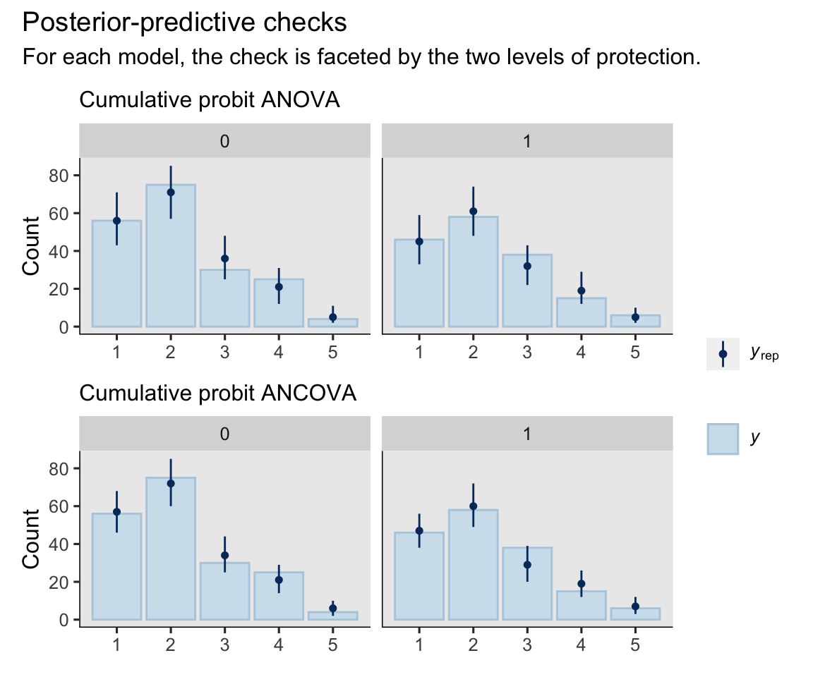
Overall, the models did pretty okay.4 It appears the baseline covaraites let the ANCOVA model make more precise predictions, which is just what we’d hope.
Theory overview
Ordinal models can make causal inference trickier than it is with other kinds of models. Volfovsky et al. ( 2015) introduced the topic well:
The first step when attempting any causal analysis is the choice of an estimand, or inferential target, which is the object of interest. When outcomes are continuous, the most commonly studied estimand is the average treatment effect (e.g., see Holland, 1986; Rubin, 1974). However, this quantity is not well defined for non-numeric data as the notion of an average of more than two ordinal values is not well defined. Other measures of centrality might be of interest; for example, the modal difference between treatment and control describes the most common number of categories that are changed due to treatment. (p. 4)
In this post, we will cover two of the approaches I have seen discussed in the literature, and I will offer a third of my own. They will be
\(\tau_z^\text{ATE}\), the average treatment effect for latent potential outcomes ( Volfovsky et al., 2015);\(\Delta_j^\text{ATE}\), the difference in probability for each of the\(J\)Likert response options ( Boes, 2013); and\(\tau_y^\text{ATE}\), the average treatment effect after transforming the ordinal model to a continuous scale.
We’ll start off with latent potential outcomes.
Latent potential outcomes and \(\tau_z^\text{ATE}\).
Sometimes we think of ordinal data as coarse measurements of a continuous underlying latent variable (
Bürkner & Vuorre, 2019;
Gelman et al., 2020, Chapter 13). In the case of our cumulative probit models, the latent variable is expressed as a standard normal distribution, which we might call \(Z\).5 Thus instead of the conventional formula
$$ \tau_\text{ATE} = \mathbb E (y_i^1 - y_i^0) = \mathbb E (y_i^1) - \mathbb E (y_i^0), $$
which is expressed in terms of the measured variable \(Y\) itself, we might instead write
$$ \tau_{\color{blueviolet}{z}}^\text{ATE} = \mathbb E ({\color{blueviolet}{z}}_i^1 - {\color{blueviolet}{z}}_i^0) = \mathbb E ({\color{blueviolet}{z}}_i^1) - \mathbb E ({\color{blueviolet}{z}}_i^0), $$
which is expressed in terms of the continuous latent variable underlying the observations of our coarsely-measured ordinal variable.
We can go beyond the simple ANOVA-style of analysis and add baseline covariates. As has been our convention from earlier posts, let \(\mathbf C_i\) stand for a vector of continuous covariates and let \(\mathbf D_i\) stand for a vector of discrete covariates, both of which vary across the \(i\) cases. We can use these to help estimate the ATE with the formula
$$ \tau_z^\text{ATE} = \mathbb E (z_i^1 - z_i^0 \mid \mathbf C_i, \mathbf D_i). $$
In words, this means the average treatment effect for the latent variable in the population is the same as the average of each person’s individual treatment effect on the latent variable, computed conditional on their continuous covariates \(\mathbf C_i\) and discrete covariates \(\mathbf D_i\). This, again, is sometimes called standardization or g-computation.
We can also use an alternative approach,
$$ \tau_z^\text{ATE} = \operatorname{\mathbb{E}}(z_i^1 \mid \mathbf C = \mathbf c, \mathbf D = \mathbf d) - \operatorname{\mathbb{E}}(z_i^0 \mid \mathbf C = \mathbf c, \mathbf D = \mathbf d), $$
where \(\mathbf C = \mathbf c\) is meant to convey you have chosen particular values \(\mathbf c\) for the variables in the \(\mathbf C\) vector, and \(\mathbf D = \mathbf d\) is meant to convey you have chosen particular values \(\mathbf d\) for the variables in the \(\mathbf D\) vector. Thus when we take \(\tau_z^\text{ATE}\) for our estimand, and we add baseline covariates to the model
$$
\begin{align*} \tau_z^\text{ATE} & = \mathbb E (z_i^1 - z_i^0 \mid \mathbf C_i, \mathbf D_i) \\ & = \operatorname{\mathbb{E}}(z_i^1 \mid \mathbf C = \mathbf c, \mathbf D = \mathbf d) - \operatorname{\mathbb{E}}(z_i^0 \mid \mathbf C = \mathbf c, \mathbf D = \mathbf d), \end{align*}
$$
which is a computational convenience we’ve only occasionally enjoyed during this blog series.6
\(\beta_1\) and latent potential outcomes.
Let’s take another focused look at the summary for \(\beta_1\) in the two models.
rbind(
  fixef(fit1)["protection", ],
  fixef(fit2)["protection", ]
) %>%
  data.frame() %>%
  mutate(model = c("ANOVA", "ANOCVA")) %>%
  select(model, everything())
##    model   Estimate Est.Error       Q2.5     Q97.5
## 1  ANOVA 0.05788666 0.1121175 -0.1640119 0.2736609
## 2 ANOCVA 0.03045630 0.1262693 -0.2165631 0.2755442
With the cumulative probit model, adding predictive baseline covariates increased the posterior SD for \(\beta_1\). From an interpretative standpoint,
$$\beta_1 = \tau_z^\text{ATE},$$
the average treatment effect on the scale of the underlying latent variable. Since we are using a cumulative probit model, this is on a standard normal (i.e., \(z\)) scale, and thus this can be interpreted as a latent Cohen’s \(d\). I believe this is the first time we’ve had a model where baseline covariates increased the posterior SD for \(\hat \beta_1\) AND the posterior SD for our causal estimate \(\hat \tau_\text{ATE}\).7 Strange, eh?
\(\mathbb E (z_i^1 - z_i^0)\) without and with covariates.
We will use standardization to compute our estimate for \(\tau_z^\text{ATE}\) via the \(\mathbb E (z_i^1 - z_i^0)\) method. For our brm() models, we can do with with fitted()- add_linpred_draws()-, or marginaleffects-based workflows. We’ll start with a fitted()-based approach. As a first step, we’ll make a predictor grid with each participants’ prez value, and counterfactual values for the independent variable protection.
# update the data grid
nd_id <- coyne2022 %>%
  select(id, male, prez) %>%
  expand_grid(protection = 0:1) %>%
  mutate(row = 1:n())

# what?
glimpse(nd_id)
## Rows: 706
## Columns: 5
## $ id         <int> 1, 1, 3, 3, 9, 9, 11, 11, 12, 12, 13, 13, 21, 21, 22, 22, 24, 24, 25, 25, 28, 28, 32, 32,…
## $ male       <dbl> 0, 0, 1, 1, 0, 0, 0, 0, 0, 0, 1, 1, 1, 1, 1, 1, 0, 0, 0, 0, 1, 1, 1, 1, 0, 0, 0, 0, 1, 1,…
## $ prez       <dbl> 2.3284981, 2.3284981, 1.4456196, 1.4456196, 1.4456196, 1.4456196, 0.5627412, 0.5627412, 1…
## $ protection <int> 0, 1, 0, 1, 0, 1, 0, 1, 0, 1, 0, 1, 0, 1, 0, 1, 0, 1, 0, 1, 0, 1, 0, 1, 0, 1, 0, 1, 0, 1,…
## $ row        <int> 1, 2, 3, 4, 5, 6, 7, 8, 9, 10, 11, 12, 13, 14, 15, 16, 17, 18, 19, 20, 21, 22, 23, 24, 25…
The trick to getting the counterfactual predictions on the latent-variable scale is to set scale = "linear" within fitted(). Here’s what the first six rows look like, using the default summary = TRUE setting.
fitted(fit1,
       newdata = nd_id,
       scale = "linear") %>%
  head()
##        Estimate Est.Error       Q2.5     Q97.5
## [1,] 0.00000000 0.0000000  0.0000000 0.0000000
## [2,] 0.05788666 0.1121175 -0.1640119 0.2736609
## [3,] 0.00000000 0.0000000  0.0000000 0.0000000
## [4,] 0.05788666 0.1121175 -0.1640119 0.2736609
## [5,] 0.00000000 0.0000000  0.0000000 0.0000000
## [6,] 0.05788666 0.1121175 -0.1640119 0.2736609
Since the ANOVA model has no way to make use of the baseline covariate prez, the counterfactual estimates are identical across participants, within each level of protection. Now we’ll show the full code necessary for the \(\mathbb E (z_i^1 - z_i^0)\) method. Note how we set summary = FALSE within fitted(). Since this code block is long, I’ll provide more annotation than usual.
# compute the posterior predictions
fitted(fit1,
       newdata = nd_id,
       scale = "linear",
       summary = F) %>%
  # convert the results to a data frame
  data.frame() %>%
  # rename the columns
  set_names(pull(nd_id, row)) %>%
  # add a numeric index for the MCMC draws
  mutate(draw = 1:n()) %>%
  # convert to the long format
  pivot_longer(-draw) %>%
  # convert the row column from the character to the numeric format
  mutate(row = as.double(name)) %>%
  # join the nd_id predictor grid to the output
  left_join(nd_id, by = "row") %>%
  # drop two of the unnecessary columns
  select(-name, -row) %>%
  # convert to a wider format so we can compute the contrast
  pivot_wider(names_from = protection, values_from = value) %>%
  # compute the ATE contrast
  mutate(tau = `1` - `0`) %>%
  # compute the average ATE value within each MCMC draw
  group_by(draw) %>%
  summarise(ate = mean(tau)) %>%
  # remove the draw index column
  select(ate) %>%
  # now summarize the ATE across the MCMC draws
  summarise(m = mean(ate),
            s = sd(ate),
            ll = quantile(ate, probs = .025),
            ul = quantile(ate, probs = .975))
## # A tibble: 1 × 4
##        m     s     ll    ul
##    <dbl> <dbl>  <dbl> <dbl>
## 1 0.0579 0.112 -0.164 0.274
As we said in the last section, \(\beta_1\) is an estimator of \(\tau_Z^\text{ATE}\) for the ordinal ANOVA model. And indeed, these summary values are identical with the summary values for \(\beta_1\). To make the same computation with the avg_comparisons() function, make sure to set type = "link".
# change the marginaleffects default to use the mean, rather than the median
options(marginaleffects_posterior_center = mean)

# compute
avg_comparisons(fit1, type = "link") %>%
  data.frame()
##         term contrast   estimate   conf.low conf.high
## 1 protection    1 - 0 0.05788666 -0.1640119 0.2736609
Happily, the summary results from avg_comparisons() match the results we got from fitted(). These methods will work much the same for the cumulative probit ANCOVA fit2. Here’s the fitted() approach.
# this line right here is the only new line
fitted(fit2,
       newdata = nd_id,
       scale = "linear",
       summary = F) %>%
  data.frame() %>%
  set_names(pull(nd_id, row)) %>%
  mutate(draw = 1:n()) %>%
  pivot_longer(-draw) %>%
  mutate(row = as.double(name)) %>%
  left_join(nd_id, by = "row") %>%
  select(-name, -row) %>%
  pivot_wider(names_from = protection, values_from = value) %>%
  mutate(tau = `1` - `0`) %>%
  group_by(draw) %>%
  summarise(ate = mean(tau)) %>%
  select(ate) %>%
  summarise(m = mean(ate),
            s = sd(ate),
            ll = quantile(ate, probs = .025),
            ul = quantile(ate, probs = .975))
## # A tibble: 1 × 4
##        m     s     ll    ul
##    <dbl> <dbl>  <dbl> <dbl>
## 1 0.0305 0.126 -0.217 0.276
Again, note how the ANCOVA results have a larger SD compared to the ANOVA results. Sigh. To compute these estimate summaries with the avg_comparisons() function, we just need to specify which variable we want the counterfactual contrast for with the variables argument.
avg_comparisons(fit2, variables = "protection", type = "link") %>%
  data.frame()
##         term contrast  estimate   conf.low conf.high
## 1 protection    1 - 0 0.0304563 -0.2165631 0.2755442
As has become our custom, it might help bring this all down to earth if we make a plot of the person-level counterfactual predictions and their contrasts for the ANCOVA model. Since the full \(N = 353\) data set would make for an overly dense plot, we’ll highlight a random \(n = 50\) subset instead. Here we select our subset, and save their id levels as a vector namedrandom_50.
set.seed(7)

random_50 <- coyne2022 %>%
  slice_sample(n = 50) %>%
  arrange(id) %>%
  pull(id)

# what is this?
print(random_50)
##  [1]   9  50  53  69  70  84 113 121 146 151 182 192 213 218 236 246 254 271 305 349 351 356 360 369 380 381
## [27] 401 405 431 452 456 485 497 511 514 543 550 555 568 575 577 582 584 588 590 595 598 636 637 638
Now plot the counterfactual latent predictions, and their contrasts, for our random \(n = 50\) subset. For the sake of practice, we’ll use a tidybayes-based workflow for the predictions. In the past we have relied on the add_epred_draws() function, but in this case since we want the predictions on the latent scale, we use the add_linpred_draws() function instead.
# counterfactual predictions
p1 <- nd_id %>%
  filter(id %in% random_50) %>%
  add_linpred_draws(fit2) %>%
  mutate(y = ifelse(protection == 0, "hat(italic(z))^0", "hat(italic(z))^1")) %>%
  group_by(id, y) %>%
  mean_qi(.linpred) %>%

  ggplot(aes(x = .linpred, y = reorder(id, .linpred), color = y)) +
  geom_interval(aes(xmin = .lower, xmax = .upper),
                position = position_dodge(width = -0.2),
                size = 1/5) +
  geom_point(aes(shape = y),
             size = 2) +
  scale_color_viridis_d(NULL, option = "A", begin = .3, end = .6,
                        labels = scales::parse_format()) +
  scale_shape_manual(NULL, values = c(20, 18),
                     labels = scales::parse_format()) +
  scale_y_discrete(breaks = NULL) +
  labs(subtitle = "Counterfactual predictions",
       x = expression(italic(Z)~(underlying~latent~variable)),
       y = "id (ranked)") +
  coord_cartesian(xlim = c(-2, 4)) +
  theme(legend.background = element_blank(),
        legend.position = c(.9, .85))

# treatment effects
p2 <- nd_id %>%
  filter(id %in% random_50) %>%
  add_linpred_draws(fit2) %>%
  ungroup() %>%
  select(id, protection, .draw, .linpred) %>%
  pivot_wider(names_from = protection, values_from = .linpred) %>%
  mutate(d = `1` - `0`) %>%
  group_by(id) %>%
  mean_qi(d) %>%

  ggplot(aes(x = d, y = reorder(id, d))) +
  geom_vline(xintercept = 0, color = "white") +
  geom_interval(aes(xmin = .lower, xmax = .upper),
                position = position_dodge(width = -0.25),
                size = 1/5, color = "black") +
  geom_point() +
  scale_y_discrete(breaks = NULL) +
  labs(subtitle = "Treatment effects",
       x = expression(hat(tau)[italic(zi)]~("i.e., "*hat(italic(z))[italic(i)]^1-hat(italic(z))[italic(i)]^0)),
       y = NULL) +
  xlim(-3, 3)

# combine and entitle
p1 + p2 +
  plot_annotation(title = "Latent person-level estimates based on the cumulative probit ANCOVA",
                  subtitle = "To reduce visual density, these are for a random subset of 50 participants.")
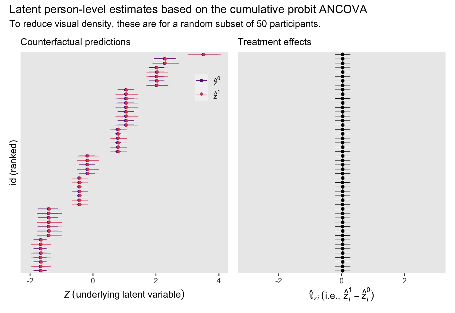
In the case of the cumulative probit ANCOVA, the latent \(z_i^1 - z_i^0\) contrasts are the same across participants, even though their individual \(z_i^1\) and \(z_i^0\) estimates differ. Here’s a closer look at the numeric summaries for the contrasts for our \(n = 50\) subset.
nd_id %>%
  filter(id %in% random_50) %>%
  add_linpred_draws(fit2) %>%
  ungroup() %>%
  select(id, protection, .draw, .linpred) %>%
  pivot_wider(names_from = protection, values_from = .linpred) %>%
  mutate(d = `1` - `0`) %>%
  group_by(id) %>%
  summarise(m = mean(d),
            s = sd(d),
            ll = quantile(d, probs = .025),
            ul = quantile(d, probs = .975))
## # A tibble: 50 × 5
##       id      m     s     ll    ul
##    <int>  <dbl> <dbl>  <dbl> <dbl>
##  1     9 0.0305 0.126 -0.217 0.276
##  2    50 0.0305 0.126 -0.217 0.276
##  3    53 0.0305 0.126 -0.217 0.276
##  4    69 0.0305 0.126 -0.217 0.276
##  5    70 0.0305 0.126 -0.217 0.276
##  6    84 0.0305 0.126 -0.217 0.276
##  7   113 0.0305 0.126 -0.217 0.276
##  8   121 0.0305 0.126 -0.217 0.276
##  9   146 0.0305 0.126 -0.217 0.276
## 10   151 0.0305 0.126 -0.217 0.276
## # ℹ 40 more rows
The contrast for each case \((\tau_{zi})\) is the same as our estimate for the overall estimand \(\tau_z^\text{ATE}\) from above. Each one is also identical with the ANCOVA model’s \(\beta_1\) parameter.
\(\mathbb E (z_i^1) - \mathbb E (z_i^0)\) without and with covariates.
The \(\mathbb E (z_i^1) - \mathbb E (z_i^0)\) method greatly simplifies the computation code. For our cumulative probit ANOVA, we just need a 2-row 1-column predictor grid for the two levels of protection.
# define the predictor grid
nd <- tibble(protection = 0:1)

fitted(fit1,
       newdata = nd,
       scale = "linear")
##        Estimate Est.Error       Q2.5     Q97.5
## [1,] 0.00000000 0.0000000  0.0000000 0.0000000
## [2,] 0.05788666 0.1121175 -0.1640119 0.2736609
Because of the identification constraint that \(\beta_0 = 0\), the group mean \(\mathbb E (z_i^0)\) is exactly zero. This simplifies our contrast of interest like so:
$$
\begin{align*} \tau_z^\text{ATE} & = \mathbb E (z_i^1) - \mathbb E (z_i^0) \\ & = \mathbb E (z_i^1) - 0 \\ & = \mathbb E (z_i^1). \end{align*}
$$
To rehearse the point again, another consequence of this parameterization is \(\mathbb E (z_i^1)\) is the same as the \(\beta_1\) parameter. Thus for our cumulative probit ANOVA
$$ \tau_z^\text{ATE} = \mathbb E (z_i^1) = {\color{blueviolet}{\beta_1}}. $$
The same is true for our cumulative probit ANCOVA. To give a sense, let’s make predictor grid with several different levels of male and prez.
nd_cate <- crossing(
  male = 0:1,
  prez = -4:4) %>%
  mutate(case = 1:n()) %>%
  expand_grid(protection = 0:1)

# what?
glimpse(nd_cate)
## Rows: 36
## Columns: 4
## $ male       <int> 0, 0, 0, 0, 0, 0, 0, 0, 0, 0, 0, 0, 0, 0, 0, 0, 0, 0, 1, 1, 1, 1, 1, 1, 1, 1, 1, 1, 1, 1,…
## $ prez       <int> -4, -4, -3, -3, -2, -2, -1, -1, 0, 0, 1, 1, 2, 2, 3, 3, 4, 4, -4, -4, -3, -3, -2, -2, -1,…
## $ case       <int> 1, 1, 2, 2, 3, 3, 4, 4, 5, 5, 6, 6, 7, 7, 8, 8, 9, 9, 10, 10, 11, 11, 12, 12, 13, 13, 14,…
## $ protection <int> 0, 1, 0, 1, 0, 1, 0, 1, 0, 1, 0, 1, 0, 1, 0, 1, 0, 1, 0, 1, 0, 1, 0, 1, 0, 1, 0, 1, 0, 1,…
Now we have our nd_cate predictor grid, we’re ready to compute the counterfactual latent predictions with the marginaleffects::predictions() function, and then plot.
predictions(fit2, newdata = nd_cate, type = "link", by = c("case", "protection", "male", "prez")) %>%
  data.frame() %>%
  mutate(y = ifelse(protection == 0, "hat(italic(z))^0", "hat(italic(z))^1")) %>%

  ggplot(aes(x = estimate, y = reorder(case, estimate), color = y)) +
  geom_interval(aes(xmin = conf.low, xmax = conf.high),
                position = position_dodge(width = -0.2),
                size = 1/5) +
  geom_point(aes(shape = y),
             size = 2) +
  scale_color_viridis_d(NULL, option = "A", begin = .3, end = .6,
                        labels = scales::parse_format()) +
  scale_shape_manual(NULL, values = c(20, 18),
                     labels = scales::parse_format()) +
  scale_y_discrete(breaks = NULL) +
  labs(title = "Counterfactual predictions (given different levels of male and prez)",
       x = expression(italic(Z)~(underlying~latent~variable)),
       y = "case (ranked)") +
  coord_cartesian(xlim = c(-6, 6)) +
  theme(legend.background = element_blank(),
        legend.position = c(.9, .78))
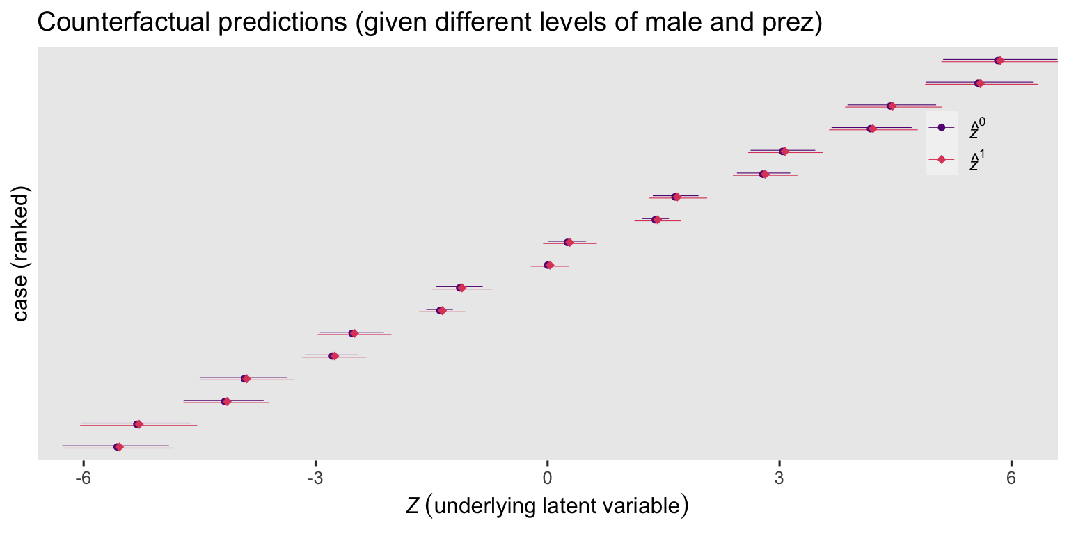
Even though the predictions vary a lot based on the given values for male and prez, their contrasts are all the same. Here we’ll explicitly compute the contrasts with the comparisons() function.
comparisons(fit2,
            newdata = nd_cate,
            type = "link",
            variables = "protection",
            by = c("case", "male", "prez"))
##
##        Term          Contrast case male prez Estimate  2.5 % 97.5 %
##  protection mean(1) - mean(0)    1    0   -4   0.0305 -0.217  0.276
##  protection mean(1) - mean(0)    2    0   -3   0.0305 -0.217  0.276
##  protection mean(1) - mean(0)    3    0   -2   0.0305 -0.217  0.276
##  protection mean(1) - mean(0)    4    0   -1   0.0305 -0.217  0.276
##  protection mean(1) - mean(0)    5    0    0   0.0305 -0.217  0.276
##  protection mean(1) - mean(0)    6    0    1   0.0305 -0.217  0.276
##  protection mean(1) - mean(0)    7    0    2   0.0305 -0.217  0.276
##  protection mean(1) - mean(0)    8    0    3   0.0305 -0.217  0.276
##  protection mean(1) - mean(0)    9    0    4   0.0305 -0.217  0.276
##  protection mean(1) - mean(0)   10    1   -4   0.0305 -0.217  0.276
##  protection mean(1) - mean(0)   11    1   -3   0.0305 -0.217  0.276
##  protection mean(1) - mean(0)   12    1   -2   0.0305 -0.217  0.276
##  protection mean(1) - mean(0)   13    1   -1   0.0305 -0.217  0.276
##  protection mean(1) - mean(0)   14    1    0   0.0305 -0.217  0.276
##  protection mean(1) - mean(0)   15    1    1   0.0305 -0.217  0.276
##  protection mean(1) - mean(0)   16    1    2   0.0305 -0.217  0.276
##  protection mean(1) - mean(0)   17    1    3   0.0305 -0.217  0.276
##  protection mean(1) - mean(0)   18    1    4   0.0305 -0.217  0.276
##
## Columns: term, contrast, case, male, prez, estimate, conf.low, conf.high, predicted, predicted_hi, predicted_lo, tmp_idx
For each combination of the baseline covariates male and prez, the result is the same when we take the average over the participants for \(\tau_z^\text{ATE}\). Here’s what that looks like when computed by the avg_comparisons() function.
avg_comparisons(fit2, variables = "protection", type = "link")
##
##        Term Contrast Estimate  2.5 % 97.5 %
##  protection    1 - 0   0.0305 -0.217  0.276
##
## Columns: term, contrast, estimate, conf.low, conf.high
These are also the same as the summary for the ANCOVA \(\beta_1\) parameter.
fixef(fit2)["protection", ]
##   Estimate  Est.Error       Q2.5      Q97.5
##  0.0304563  0.1262693 -0.2165631  0.2755442
Thus for the cumulative probit ANCOVA
$$
\begin{align*} \tau_z^\text{ATE} & = \mathbb E (z_i^1 - z_i^0 \mid \mathbf C_i, \mathbf D_i) \\ & =\operatorname{\mathbb{E}}(z_i^1 \mid \mathbf C = \mathbf c, \mathbf D = \mathbf d) - \operatorname{\mathbb{E}}(z_i^0 \mid \mathbf C = \mathbf c, \mathbf D = \mathbf d) \\ & = \beta_1. \end{align*}
$$
Latent wrap-up.
Volfovsky et al’s latent potential outcomes approach has a few attractive properties. It allows researchers to estimate the latent potential outcomes, and their contrasts, for all participants. Because latent variables are numeric, it also allows researchers to compute an ATE on the latent scale. However, latent variable theory might not fit well with all substantive research programs, and some researchers may prefer their effect sizes to have a closer resemblance to the underlying data. Finally, the latent potential outcomes approach does not seem to benefit from baseline covariates, which is something I have not seen acknowledged in the causal inference methodological literature yet.
Conditional probabilities for each response option and \(\Delta_j^\text{ATE}\).
We can take very different approach by computing a treatment effect defined in terms of the probabilities of the given Likert response options. Boes (
2013) referred to this effect size as \(\Delta_y^\text{ATE}\). Frankly, I find Boes’s notation slightly opaque, and I’m going to refer to his version of the ATE throughout this post as \(\Delta_{\color{blueviolet}{j}}^\text{ATE}\), which is meant to more explicitly connect the effect size with a given level of the \(J\) ordered response options. We might define \(\Delta_j^\text{ATE}\) as
$$ \Delta_j^\text{ATE} = \Pr (y_i^1 = j) - \Pr(y_i^0 = j), \text{ for } j = 1, \dots, J. $$
In words, this is the probability of the \(j\)th Likert response for those in the treatment condition minus the probability of the \(j\)th Likert response for those in the treatment condition. Instead of a single effect size, this will end up returning \(J\) treatment effects. To make that more explicit, we might express the \(\Delta_j^\text{ATE}\) measures for our 5 levels of post as
$$
\begin{align*} \Delta_{\color{blueviolet}{1}}^\text{ATE} & = \Pr (y_i^1 = {\color{blueviolet}{1}}) - \Pr(y_i^0 = {\color{blueviolet}{1}}) \\ \Delta_{\color{blueviolet}{2}}^\text{ATE} & = \Pr (y_i^1 = {\color{blueviolet}{2}}) - \Pr(y_i^0 = {\color{blueviolet}{2}}) \\ \Delta_{\color{blueviolet}{3}}^\text{ATE} & = \Pr (y_i^1 = {\color{blueviolet}{3}}) - \Pr(y_i^0 = {\color{blueviolet}{3}}) \\ \Delta_{\color{blueviolet}{4}}^\text{ATE} & = \Pr (y_i^1 = {\color{blueviolet}{4}}) - \Pr(y_i^0 = {\color{blueviolet}{4}}) \\ \Delta_{\color{blueviolet}{5}}^\text{ATE} & = \Pr (y_i^1 = {\color{blueviolet}{5}}) - \Pr(y_i^0 = {\color{blueviolet}{5}}). \end{align*}
$$
Since our ordinal models return a \(\mathbf p\) vector of probabilities, \(\{p_1, p_2, p_3, p_4, p_5 \}\), we could also express this in the more compact notation of
$$ \Delta_j^\text{ATE} = {\color{blueviolet}{p_j^1 - p_j^0}}, \text{ for } j = 1, \dots, J. $$
Further, since our regression format will also allow us to compute person-specific counterfactual estimates for \(p_{ij}^1\) and \(p_{ij}^0\), we can expand the framework to
$$ \Delta_j^\text{ATE} = {\color{blueviolet}{\mathbb E_j (p_{ij}^1 - p_{ij}^0)}} = p_j^1 - p_j^0, $$
where \(p_{ij}^1 - p_{ij}^0\) is the counterfactual person-specific difference in probability for a given Likert response option, based on whether they were in treatment or control.
We can go beyond the simple ANOVA-style of analysis and add baseline covariates. Let \(\mathbf C_i\) stand for a vector of continuous covariates and \(\mathbf D_i\) stand for a vector of discrete covariates, both of which vary across the \(i\) cases. We can use these to help estimate \(\Delta_j^\text{ATE}\) with the formula,
$$
\Delta_j^\text{ATE} = \mathbb E_j (p_{ij}^1 - p_{ij}^0 \mid \mathbf C_i, \mathbf D_i).
$$
In words, we can compute average treatment effect of the probability difference of observing a particular Likert response with and without the treatment \((\Delta_j^\text{ATE})\) by averaging all the person-specific probability differences of observing a particular Likert response with and without the treatment \((p_{ij}^1 - p_{ij}^0)\), computed conditional on their continuous covariates \(\mathbf C_i\) and discrete covariates \(\mathbf D_i\). We accomplish this averaging by the standardization or g-computation methods we’ve come to know and love. However, as has been the case in other contexts were we used a link function,
$$ {\color{blueviolet}{\Delta_j^\text{CATE}}} = \mathbb E_j (p_{ij}^1 \mid \mathbf C = \mathbf c, \mathbf D = \mathbf d) - \mathbb E_j (p_{ij}^0 \mid \mathbf C = \mathbf c, \mathbf D = \mathbf d) , $$
where \(\mathbf C = \mathbf c\) is meant to convey you have chosen particular values \(\mathbf c\) for the variables in the \(\mathbf C\) vector, and \(\mathbf D = \mathbf d\) is meant to convey you have chosen particular values \(\mathbf d\) for the variables in the \(\mathbf D\) vector. Thus when we add covariates into the model
$$ \mathbb E_j (p_{ij}^1 - p_{ij}^0 \mid \mathbf C_i, \mathbf D_i) \text{ } {\color{blueviolet}{\neq}} \text{ } \mathbb E_j (p_{ij}^1 \mid \mathbf C = \mathbf c, \mathbf D = \mathbf d) - \mathbb E_j (p_{ij}^0\mid \mathbf C = \mathbf c, \mathbf D = \mathbf d), $$
and thus
$$ \Delta_j^\text{ATE} \neq \Delta_j^\text{CATE}. $$
Okay, let’s move into application.
\(\beta_1\) and \(\Delta_j^\text{ATE}\).
To my knowledge, there is no way to compute \(\Delta_j^\text{ATE}\) based with the \(\beta_1\) parameter alone. This method requires we use the parameters from the full ordinal model. If there’s been one message throughout this blog series, it’s that one naïvely interprets \(\beta_1\) at one’s own peril. So what is \(\beta_1\) within the context of the estimand \(\Delta_j^\text{ATE}\)? It’s one small cog in a large glorious machine. Dont’ get caught up on the cogs, friends.
\(\mathbb E_j (p_{ij}^1 - p_{ij}^0)\) without and with covariates.
We will use standardization to compute our estimate for \(\Delta_j^\text{ATE}\) via the \(\mathbb E_j (p_{ij}^1 - p_{ij}^0)\) method. For our brm() models, we can do with with fitted()- add_epred_draws()-, or marginaleffects-based workflows. However, I recommend against using fitted() for computing the \(p_{ij}\) estimates from ordinal models; it makes for long complicated code. Instead, here we’ll jump straight to an add_epred_draws()-based workflow. We’ll continue using our nd_id predictor grid. Here are what the first 6 rows of the output look like for our cumulative probit ANOVA fit1:
# compute and save
fit1_conditional_probabilities_by_id <- nd_id %>%
  add_epred_draws(fit1) %>%
  ungroup()

# show the first 6 rows
fit1_conditional_probabilities_by_id %>%
  head()
## # A tibble: 6 × 11
##      id  male  prez protection   row  .row .chain .iteration .draw .category .epred
##   <int> <dbl> <dbl>      <int> <int> <int>  <int>      <int> <int> <fct>      <dbl>
## 1     1     0  2.33          0     1     1     NA         NA     1 1          0.294
## 2     1     0  2.33          0     1     1     NA         NA     2 1          0.313
## 3     1     0  2.33          0     1     1     NA         NA     3 1          0.262
## 4     1     0  2.33          0     1     1     NA         NA     4 1          0.267
## 5     1     0  2.33          0     1     1     NA         NA     5 1          0.329
## 6     1     0  2.33          0     1     1     NA         NA     6 1          0.290
Note the new .category column, which marks the five Likert response options for the outcome variable post, ranging from 1 to 5 in the output. The .epred column is the conditional probability for each of those response options, for a given participant at a given counterfactual level of protection, and for a given MCMC draw. As a consequence, the full output is very long at 14,120,000 rows. That is
$$14{,}120{,}000 \text{ rows} = 5 \text{ ratings}\times 353 \text{ cases} \times 2 \text{ levels of protection} \times 4000 \text{ MCMC draws}.$$
Here’s how to group and summarize these results to compute the summaries for the \(\Delta_j^\text{ATE}\) estimates.
# contrasts
fit1_conditional_probabilities_by_id %>%
  # subset the columns
  select(id, protection, .draw, .category, .epred) %>%
  # convert to a wider format
  pivot_wider(names_from = protection, values_from = .epred) %>%
  # compute the contrasts
  mutate(`1 - 0` = `1` - `0`) %>%
  # average the contrasts over the cases
  group_by(.draw, .category) %>%
  summarise(`1 - 0` = mean(`1 - 0`)) %>%
  # now summarize the category-level contrasts
  group_by(.category) %>%
  summarise(p = mean(`1 - 0`),
            sd = sd(`1 - 0`),
            ll = quantile(`1 - 0`, probs = .025),
            ul = quantile(`1 - 0`, probs = .975))
## `summarise()` has grouped output by '.draw'. You can override using the `.groups` argument.

## # A tibble: 5 × 5
##   .category        p      sd      ll      ul
##   <fct>        <dbl>   <dbl>   <dbl>   <dbl>
## 1 1         -0.0195  0.0380  -0.0926 0.0552
## 2 2         -0.00165 0.00390 -0.0113 0.00500
## 3 3          0.00797 0.0155  -0.0225 0.0382
## 4 4          0.00920 0.0181  -0.0268 0.0450
## 5 5          0.00397 0.00792 -0.0110 0.0203
Now compare those results with those from our cumulative probit ANCOVA, fit2.
# compute and save
fit2_conditional_probabilities_by_id <- nd_id %>%
  add_epred_draws(fit2) %>%
  ungroup()

# summarize
fit2_conditional_probabilities_by_id %>%
  select(id, protection, .draw, .category, .epred) %>%
  pivot_wider(names_from = protection, values_from = .epred) %>%
  mutate(`1 - 0` = `1` - `0`) %>%
  group_by(.draw, .category) %>%
  summarise(`1 - 0` = mean(`1 - 0`)) %>%
  group_by(.category) %>%
  summarise(p = mean(`1 - 0`),
            sd = sd(`1 - 0`),
            ll = quantile(`1 - 0`, probs = .025),
            ul = quantile(`1 - 0`, probs = .975))
## `summarise()` has grouped output by '.draw'. You can override using the `.groups` argument.

## # A tibble: 5 × 5
##   .category         p      sd       ll      ul
##   <fct>         <dbl>   <dbl>    <dbl>   <dbl>
## 1 1         -0.00617  0.0257  -0.0564  0.0438
## 2 2          0.000452 0.00217 -0.00403 0.00483
## 3 3          0.00186  0.00773 -0.0130  0.0171
## 4 4          0.00236  0.00990 -0.0171  0.0222
## 5 5          0.00150  0.00621 -0.0104  0.0140
It might be hard to catch, but the ANCOVA-based \(\Delta_j^\text{ATE}\) estimates are more precise, as indicated by their smaller posterior SD’s. Happily, we can compute these same estimates with much thriftier syntax with the handy avg_comparisons() function.
avg_comparisons(fit1, variables = "protection") # ANOVA
##
##  Group       Term Contrast Estimate   2.5 % 97.5 %
##      1 protection    1 - 0 -0.01948 -0.0926 0.0552
##      2 protection    1 - 0 -0.00165 -0.0113 0.0050
##      3 protection    1 - 0  0.00797 -0.0225 0.0382
##      4 protection    1 - 0  0.00920 -0.0268 0.0450
##      5 protection    1 - 0  0.00397 -0.0110 0.0203
##
## Columns: group, term, contrast, estimate, conf.low, conf.high
avg_comparisons(fit2, variables = "protection") # ANCOVA
##
##  Group       Term Contrast  Estimate    2.5 %  97.5 %
##      1 protection    1 - 0 -0.006169 -0.05639 0.04380
##      2 protection    1 - 0  0.000452 -0.00403 0.00483
##      3 protection    1 - 0  0.001857 -0.01297 0.01706
##      4 protection    1 - 0  0.002356 -0.01712 0.02221
##      5 protection    1 - 0  0.001503 -0.01039 0.01399
##
## Columns: group, term, contrast, estimate, conf.low, conf.high
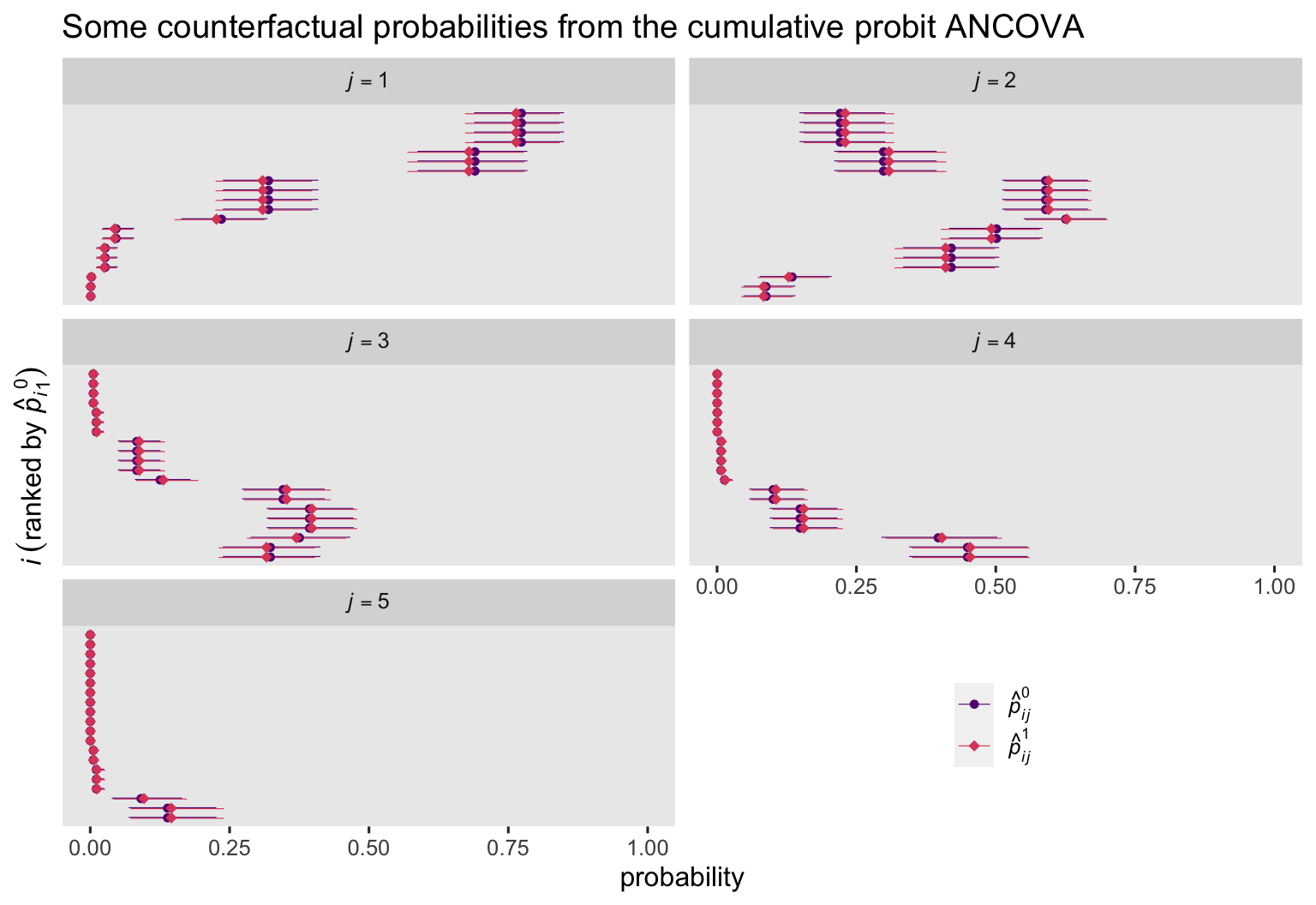
It might help clarify what we’ve been computing and summarizing if we make a couple plots. Since the conditional probabilities are the same across participants in the ANOVA model, we’ll jump straight to the cumulative probit ANCOVA. Earlier in the post, we used data from an \(n = 50\) subset. Given how we how have 10 counterfactual estimates for each case, we’ll want to use an even smaller \(n = 20\) subset.
# define the random 20 cases
set.seed(7)

random_20 <- coyne2022 %>%
  slice_sample(n = 20) %>%
  arrange(id) %>%
  pull(id)

# what?
print(random_20)
## [1] 50 53 121 192 218 246 271 305 351 381 401 431 456 550 555 575 582 595 598 637
Next we’ll need to make an index for rank ordering the cases. Since we’ll be faceting over the 5 levels of \(J\), we’ll just want to rank order for one of those levels. I choose \(j = 1\).
id_ranks <- predictions(
  fit2,
  newdata = nd_id %>% filter(id %in% random_20),
  by = c("protection", "group", "id")) %>%
  data.frame() %>%
  filter(group == 1, protection == 0) %>%
  arrange(estimate) %>%
  mutate(rank = 1:n()) %>%
  select(id, rank)

# what is this?
glimpse(id_ranks)
## Rows: 20
## Columns: 2
## $ id   <int> 192, 555, 121, 271, 381, 431, 351, 582, 53, 218, 246, 401, 456, 50, 598, 637, 305, 550, 575, 595
## $ rank <int> 1, 2, 3, 4, 5, 6, 7, 8, 9, 10, 11, 12, 13, 14, 15, 16, 17, 18, 19, 20
Now we’re finally ready to plot those \(p_{ij}^1\) and \(p_{ij}^0\) estimates for our \(n = 20\) subset.
predictions(fit2,
            newdata = nd_id %>% filter(id %in% random_20),
            by = c("protection", "group", "id")) %>%
  data.frame() %>%
  left_join(id_ranks, by = "id") %>%
  mutate(protection = ifelse(protection == 0, "hat(italic(p))[italic(ij)]^0", "hat(italic(p))[italic(ij)]^1"),
         j = str_c("italic(j)==", group)) %>%

  # plot!
  ggplot(aes(x = estimate, y = rank)) +
  geom_interval(aes(xmin = conf.low, xmax = conf.high, color = protection),
                    position = position_dodge(width = -0.2),
                    size = 1/5) +
  geom_point(aes(color = protection, shape = protection),
             size = 2) +
  scale_color_viridis_d(NULL, option = "A", begin = .3, end = .6,
                        labels = scales::parse_format()) +
  scale_shape_manual(NULL, values = c(20, 18),
                     labels = scales::parse_format()) +
  scale_x_continuous(limits = c(0, 1)) +
  scale_y_discrete(breaks = NULL) +
  labs(title = "Some counterfactual probabilities from the cumulative probit ANCOVA",
       x = "probability",
       y = expression(italic(i)~(ranked~by~hat(italic(p))[italic(i)][1]^0))) +
  theme(legend.background = element_blank(),
        legend.position = c(.75, .15)) +
  facet_wrap(~ j, labeller = label_parsed, ncol = 2)
Here’s a plot of the corresponding \(p_{ij}^1 - p_{ij}^0\) contrasts.
comparisons(fit2,
            newdata = nd_id %>% filter(id %in% random_20),
            variable = "protection",
            by = c("group", "id")) %>%
  data.frame() %>%
  left_join(id_ranks, by = "id") %>%
  mutate(j = str_c("italic(j)==", group)) %>%

  ggplot(aes(x = estimate, xmin = conf.low, xmax = conf.high, y = rank)) +
  geom_vline(xintercept = 0, color = "white") +
  geom_interval(size = 1/5) +
  geom_point(size = 1) +
  scale_x_continuous(limits = c(-0.5, 0.5)) +
  scale_y_discrete(breaks = NULL) +
  labs(title = "Some treatment effect estimates from the cumulative probit ANCOVA",
       x = expression(hat(italic(p))[italic(ij)]^1-hat(italic(p))[italic(ij)]^0),
       y = expression(italic(i)~(ranked~by~hat(italic(p))[italic(i)][1]^0))) +
  facet_wrap(~ j, labeller = label_parsed, ncol = 2)
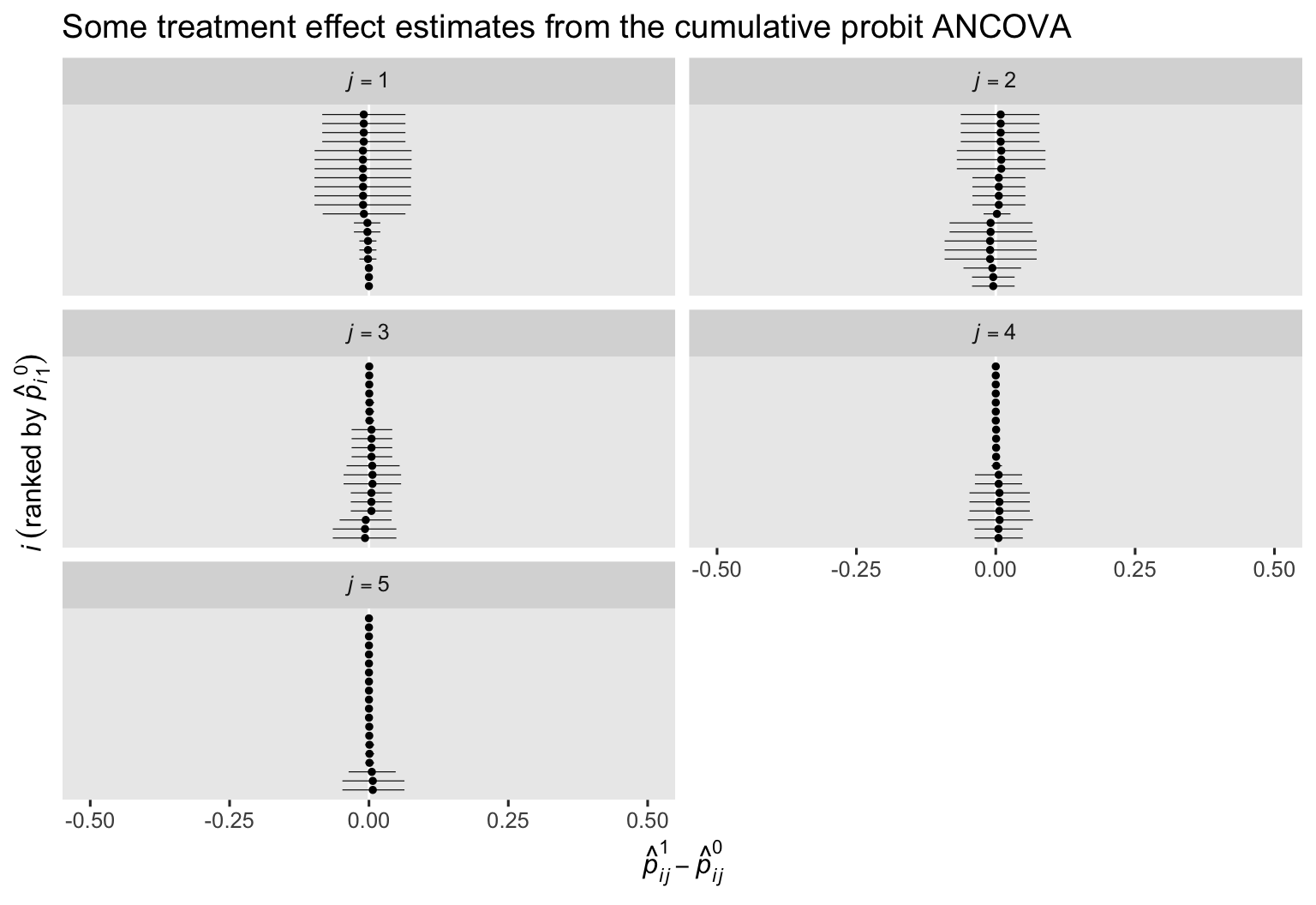
Here we see that even though the \(p_{ij}^1 - p_{ij}^0\) contrasts are pretty small across all cases, the estimates differ in terms of their posterior means (dots) and widths of their 95% intervals (horizontal lines).
\(p_j^1 - p_j^0\) without covariates.
For the \(p_j^1 - p_j^0\) method, we’ll continue to rely on the add_epred_draws()- and marginaleffects-based workflows. For our ANOVA model, we can continue using the simple nd predictor grid, which we’ll reproduce here just in case you forgot which one what was. Here are what the first 6 rows of the output look like for our cumulative probit ANOVA fit1:
# define the predictor grid
nd <- tibble(protection = 0:1)

# compute and save
fit1_conditional_probabilities_by_group <- nd %>%
  add_epred_draws(fit1) %>%
  ungroup()

# show the first 6 rows
fit1_conditional_probabilities_by_group %>%
  head()
## # A tibble: 6 × 7
##   protection  .row .chain .iteration .draw .category .epred
##        <int> <int>  <int>      <int> <int> <fct>      <dbl>
## 1          0     1     NA         NA     1 1          0.294
## 2          0     1     NA         NA     2 1          0.313
## 3          0     1     NA         NA     3 1          0.262
## 4          0     1     NA         NA     4 1          0.267
## 5          0     1     NA         NA     5 1          0.329
## 6          0     1     NA         NA     6 1          0.290
As we’re now averaging over participants, the add_epred_draws() output is only 40,000 rows long. Here’s how to summarize the \(J\) conditional probabilities and their contrasts.
# conditional probabilities
fit1_conditional_probabilities_by_group %>%
  # now summarize the category-level probabilities, by protection
  group_by(protection, .category) %>%
  summarise(p = mean(.epred),
            sd = sd(.epred),
            ll = quantile(.epred, probs = .025),
            ul = quantile(.epred, probs = .975))
## `summarise()` has grouped output by 'protection'. You can override using the `.groups` argument.

## # A tibble: 10 × 6
## # Groups:   protection [2]
##    protection .category      p      sd     ll     ul
##         <int> <fct>      <dbl>   <dbl>  <dbl>  <dbl>
##  1          0 1         0.296  0.0302  0.240  0.357
##  2          0 2         0.376  0.0264  0.326  0.427
##  3          0 3         0.190  0.0223  0.148  0.234
##  4          0 4         0.111  0.0187  0.0768 0.150
##  5          0 5         0.0281 0.00918 0.0134 0.0487
##  6          1 1         0.277  0.0317  0.218  0.342
##  7          1 2         0.374  0.0264  0.324  0.425
##  8          1 3         0.198  0.0233  0.155  0.245
##  9          1 4         0.120  0.0198  0.0836 0.162
## 10          1 5         0.0321 0.0104  0.0149 0.0552
# contrasts
fit1_conditional_probabilities_by_group %>%
  select(protection, .draw, .category, .epred) %>%
  pivot_wider(names_from = protection, values_from = .epred) %>%
  mutate(`1 - 0` = `1` - `0`) %>%
  # now summarize the category-level probabilities, by protection
  group_by(.category) %>%
  summarise(p = mean(`1 - 0`),
            sd = sd(`1 - 0`),
            ll = quantile(`1 - 0`, probs = .025),
            ul = quantile(`1 - 0`, probs = .975))
## # A tibble: 5 × 5
##   .category        p      sd      ll      ul
##   <fct>        <dbl>   <dbl>   <dbl>   <dbl>
## 1 1         -0.0195  0.0380  -0.0926 0.0552
## 2 2         -0.00165 0.00390 -0.0113 0.00500
## 3 3          0.00797 0.0155  -0.0225 0.0382
## 4 4          0.00920 0.0181  -0.0268 0.0450
## 5 5          0.00397 0.00792 -0.0110 0.0203
You can get the same results for the posterior means and 95% intervals with the predictions() and comparisons() functions.
# conditional probabilities
predictions(fit1, newdata = nd, by = c("protection", "group"))
##
##  Group protection Estimate  2.5 % 97.5 %
##      1          0   0.2960 0.2403 0.3566
##      1          1   0.2765 0.2184 0.3418
##      2          0   0.3758 0.3256 0.4269
##      2          1   0.3742 0.3236 0.4245
##      3          0   0.1896 0.1478 0.2342
##      3          1   0.1975 0.1550 0.2447
##      4          0   0.1105 0.0768 0.1504
##      4          1   0.1197 0.0836 0.1622
##      5          0   0.0281 0.0134 0.0487
##      5          1   0.0321 0.0149 0.0552
##
## Columns: group, protection, estimate, conf.low, conf.high
# conditional probability contrasts
comparisons(fit1, newdata = nd, by = "group")
##
##  Group       Term          Contrast Estimate   2.5 % 97.5 %
##      1 protection mean(1) - mean(0) -0.01948 -0.0926 0.0552
##      2 protection mean(1) - mean(0) -0.00165 -0.0113 0.0050
##      3 protection mean(1) - mean(0)  0.00797 -0.0225 0.0382
##      4 protection mean(1) - mean(0)  0.00920 -0.0268 0.0450
##      5 protection mean(1) - mean(0)  0.00397 -0.0110 0.0203
##
## Columns: group, term, contrast, estimate, conf.low, conf.high, predicted, predicted_hi, predicted_lo, tmp_idx
This method for estimating \(\Delta_j^\text{ATE}\), however, is only available for the ANOVA model. Once you add baseline covariates to the model, the \((p_j^1 \mid \mathbf C = \mathbf c, \mathbf D = \mathbf d) - (p_j^0 \mid \mathbf C = \mathbf c, \mathbf D = \mathbf d)\) method can only return some version of \(\Delta_j^\text{CATE}\), which isn’t the estimand of interest in this blog series.8
Before we move on from this section, we might depict these counterfactual probabilities and their contrasts with a plot. We’ll continue on with the compact predictions() and comparisons() syntax.
# conditional probabilities
p1 <- predictions(fit1, newdata = nd) %>%
  data.frame() %>%
  mutate(protection = ifelse(protection == 0, "italic(p[j])^0", "italic(p[j])^1")) %>%

  ggplot(aes(x = group, y = estimate, ymin = conf.low, ymax = conf.high,
             color = protection)) +
  geom_hline(yintercept = 1:4 / 10, color = "white") +
  geom_linerange(linewidth = 3/4, position = position_dodge(width = 1/3)) +
  geom_point(aes(shape = protection),
             position = position_dodge(width = 1/3),
             size = 3) +
  scale_color_viridis_d(NULL, option = "A", begin = .3, end = .6,
                        labels = scales::parse_format()) +
  scale_shape_manual(NULL, values = c(20, 18),
                     labels = scales::parse_format()) +
  scale_y_continuous("probability", limits = c(0, 0.5)) +
  labs(subtitle = "Conditional probabilities",
       x = expression(Likert~response~option~(italic(j)))) +
  theme(legend.background = element_blank(),
        legend.position = c(0.85, 0.9))

# contrasts
p2 <- comparisons(fit1, newdata = nd, by = "group") %>%
  data.frame() %>%

  ggplot(aes(x = group, y = estimate, ymin = conf.low, ymax = conf.high)) +
  geom_hline(yintercept = -2:2 / 10, color = "white") +
  geom_pointrange(linewidth = 3/4, size = 1/3) +
  scale_y_continuous(expression(italic(p[j])^1-italic(p[j])^0), limits = c(-0.25, 0.25)) +
  labs(subtitle = expression(Delta[italic(j)]^{ATE}~(contrasts)),
       x = expression(Likert~response~option~(italic(j))))

# combine and entitle
p1 + p2 + plot_annotation(title = "Cumulative probit ANOVA")
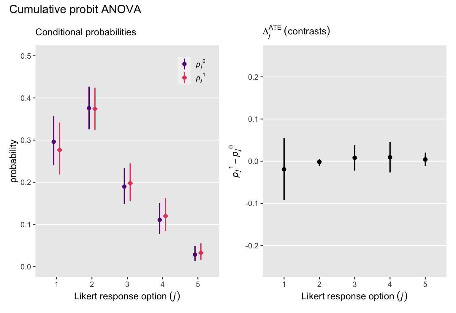
That is, the posteriors for our \(\Delta_j^\text{ATE}\) contrasts are all pretty small. The intervention was not effective.
Although we can’t make the corresponding plot with the \((p_j^1 \mid \mathbf C = \mathbf c, \mathbf D = \mathbf d) - (p_j^0 \mid \mathbf C = \mathbf c, \mathbf D = \mathbf d)\) method, we can switch back to the \(\mathbb E_j (p_{ij}^1 - p_{ij}^0 \mid \mathbf C_i, \mathbf D_i)\) method to make the contrast plot. We might further extrapolate from that method to compute the average relative probabilities for the control condition with
$$\mathbb E_j (p_{ij}^0 \mid \mathbf C_i, \mathbf D_i),$$
and average relative probabilities for the experimental condition with
$$\mathbb E_j (p_{ij}^1 \mid \mathbf C_i, \mathbf D_i).$$
Here’s what that can look like for our cumulative probit ANCOVA.
# conditional probabilities
p3 <- avg_predictions(fit2, newdata = nd_id, by = c("protection", "group")) %>%
  data.frame() %>%
  mutate(protection = ifelse(protection == 0, "E[italic(j)](hat(italic(p))[italic(ij)]^0)", "E[italic(j)](hat(italic(p))[italic(ij)]^1)")) %>%

  ggplot(aes(x = group, y = estimate, ymin = conf.low, ymax = conf.high,
             color = protection)) +
  geom_hline(yintercept = 1:4 / 10, color = "white") +
  geom_linerange(linewidth = 3/4, position = position_dodge(width = 1/3)) +
  geom_point(aes(shape = protection),
             position = position_dodge(width = 1/3),
             size = 3) +
  scale_color_viridis_d(NULL, option = "A", begin = .3, end = .6,
                        labels = scales::parse_format()) +
  scale_shape_manual(NULL, values = c(20, 18),
                     labels = scales::parse_format()) +
  scale_y_continuous("probability", limits = c(0, 0.5)) +
  labs(subtitle = "Conditional probabilities",
       x = expression(Likert~response~option~(italic(j)))) +
  theme(legend.background = element_blank(),
        legend.position = c(0.85, 0.9))

# contrasts
p4 <- avg_comparisons(fit2, variables = "protection") %>%
  data.frame() %>%

  ggplot(aes(x = group, y = estimate, ymin = conf.low, ymax = conf.high)) +
  geom_hline(yintercept = -2:2 / 10, color = "white") +
  geom_pointrange(linewidth = 3/4, size = 1/3) +
  scale_y_continuous(expression(E(italic(p[ij])^1-italic(p[ij])^0)), limits = c(-0.25, 0.25)) +
  labs(subtitle = expression(Delta[italic(j)]^{ATE}~(contrasts)),
       x = expression(Likert~response~option~(italic(j))))

# combine and entitle
p3 + p4 + plot_annotation(title = "Cumulative probit ANCOVA")
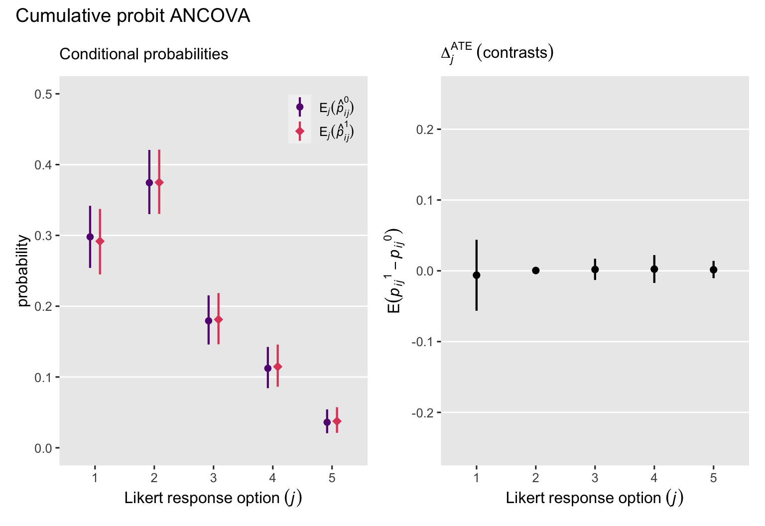
Across each of the \(J\) levels of our ordinal variable, the conditional probabilities and their contrasts are more precise when based on our cumulative probit ANCOVA model, fit2, with its nice baseline covariates. This is in sharp contrast to the latent potential outcomes results, which got less precise with the baseline covariates.
Response contrast wrap-up.
Boes’s conditional probabilities approach is nice in that it clearly connects the causal estimands to some of the primary parameters in the statistical model \((\mathbb p)\), and it emphasizes the ordinal nature of the dependent variable. This approach also benefits from high-quality baseline covariates. The multidimensional nature of the causal estimand \(\Delta_j^\text{ATE}\) seems mixed. On the one hand, this approach seems more sophisticated than an overall summary. On the other hand, a multidimensional estimand may make it harder to communicate the primary results to audiences not filled with stats geeks.
\(\tau_y^\text{ATE}\): Differences in ordinal items summarized as continuous.
Substantive researchers often summarize ordinal variables with means and standard deviations, much like they would with truly continuous variables. Though this practice is not statistically rigorous, many substantive researchers find this meaningful. It turns out there’s a known way to compute the “mean” of an ordinal variable using the parameters of an ordinal model, and it’s pretty simple. Say you have some ordinal variable called rating, with \(J\) response options, and \(p_j\) denoting the probability for a given option. You can compute the mean with the equation
$$\mathbb E(\text{rating}) = \sum_1^J p_j \times j,$$
which is just a formal way of saying the mean for your ordinal rating variable is the same as the sum of the \(p_j\) probabilities multiplied by their \(j\) response values. If our rating variable ranged from 1 to 4, and each of those values was equally probable, here’s how we’d compute the mean.
tibble(j = 1:4) %>%
  mutate(pj = .25) %>%
  mutate(`pj * j` = pj * j) %>%
  summarise(mean = sum(`pj * j`))
## # A tibble: 1 × 1
##    mean
##   <dbl>
## 1   2.5
Run that little code block step by step to make sure you follow. Since our cumulative probit models return the full \(\mathbb p\) vector of probabilities, we can use them to compute conditional means with this approach. Not only can we compute conditional means at the group level, \(\mathbb E (y_i^1)\) and \(\mathbb E (y_i^0)\), we could also compute conditional expectations at the participant level, \(\hat y_i^1\) and \(\hat y_i^0\). Thus, we might use this method to make causal inferences with the equation
$$ \tau_y^\text{ATE} = \mathbb E (y_i^1 - y_i^0) = \mathbb E (y_i^1) - \mathbb E (y_i^0), $$
where \(\tau_y^\text{ATE}\) is the average treatment effect expressed as if the ordinal variable was continuous. We can then generalize this approach to include baseline covariates with the equation
$$ \tau_y^\text{ATE} = \mathbb E (y_i^1 - y_i^0 \mid \mathbf C_i, \mathbf D_i). $$
Let’s see how this could work in practice.
\(\beta_1\) and \(\tau_y^\text{ATE}\).
To my knowledge, there is no way to compute \(\tau_y^\text{ATE}\) based with the \(\beta_1\) parameter alone. This method requires we use the parameters from the full ordinal model.
\(\mathbb E (y_i^1 - y_i^0)\) without and with covariates.
We will use standardization to compute \(\tau_y^\text{ATE}\) via the \(\mathbb E (y_i^1 - y_i^0)\) method. For our brm() models, we can do this with fitted()- or add_epred_draws()-based workflows. However, I recommend we focus on the add_epred_draws() approach, as the fitted() approach will make for overly complex code. For this method, we start with a full predictor grid with each participants’ prez value, and counterfactual values for the independent variable protection. We’ve already saved such a grid as nd_id. Here’s another look.
# update the data grid
nd_id <- coyne2022 %>%
  select(id, male, prez) %>%
  expand_grid(protection = 0:1) %>%
  mutate(row = 1:n())

# what?
glimpse(nd_id)
## Rows: 706
## Columns: 5
## $ id         <int> 1, 1, 3, 3, 9, 9, 11, 11, 12, 12, 13, 13, 21, 21, 22, 22, 24, 24, 25, 25, 28, 28, 32, 32,…
## $ male       <dbl> 0, 0, 1, 1, 0, 0, 0, 0, 0, 0, 1, 1, 1, 1, 1, 1, 0, 0, 0, 0, 1, 1, 1, 1, 0, 0, 0, 0, 1, 1,…
## $ prez       <dbl> 2.3284981, 2.3284981, 1.4456196, 1.4456196, 1.4456196, 1.4456196, 0.5627412, 0.5627412, 1…
## $ protection <int> 0, 1, 0, 1, 0, 1, 0, 1, 0, 1, 0, 1, 0, 1, 0, 1, 0, 1, 0, 1, 0, 1, 0, 1, 0, 1, 0, 1, 0, 1,…
## $ row        <int> 1, 2, 3, 4, 5, 6, 7, 8, 9, 10, 11, 12, 13, 14, 15, 16, 17, 18, 19, 20, 21, 22, 23, 24, 25…
We’ve already saved the initial add_epred_draws()-based code in a previous section. We saved the ANOVA results as fit1_conditional_probabilities_by_id and the ANCOVA results as fit2_conditional_probabilities_by_id. Using the fit1_conditional_probabilities_by_id object as a starting point, here’s how we might then use our ordinal ANOVA to compute participant-level \(\hat y_i^1\) and \(\hat y_i^0\) estimates, and their contrasts.
# conditional expectations
fit1_conditional_probabilities_by_id %>%
  # convert the .category factor to numeric
  mutate(j = as.double(.category)) %>%
  # compute p[j] * j
  mutate(product = j * .epred) %>%
  # group and convert to the y_hat metric
  group_by(id, protection, .draw) %>%
  summarise(y_hat = sum(product)) %>%
  # summarize
  group_by(id, protection) %>%
  mean_qi(y_hat) %>%
  # just show the first 6 rows
  head()
## # A tibble: 6 × 8
##      id protection y_hat .lower .upper .width .point .interval
##   <int>      <int> <dbl>  <dbl>  <dbl>  <dbl> <chr>  <chr>
## 1     1          0  2.20   2.05   2.35   0.95 mean   qi
## 2     1          1  2.26   2.10   2.42   0.95 mean   qi
## 3     3          0  2.20   2.05   2.35   0.95 mean   qi
## 4     3          1  2.26   2.10   2.42   0.95 mean   qi
## 5     9          0  2.20   2.05   2.35   0.95 mean   qi
## 6     9          1  2.26   2.10   2.42   0.95 mean   qi
# contrasts
fit1_conditional_probabilities_by_id %>%
  # convert the .category factor to numeric
  mutate(j = as.double(.category)) %>%
  # compute p[j] * j
  mutate(product = j * .epred) %>%
  # group and convert to the y_hat metric
  group_by(id, protection, .draw) %>%
  summarise(y_hat = sum(product)) %>%
  # convert to the wide format with respect to protection
  pivot_wider(names_from = protection, values_from = y_hat) %>%
  # compute the protection contrast
  mutate(`1 - 0` = `1` - `0`) %>%
  # group and summarize by id
  group_by(id) %>%
  mean_qi(`1 - 0`) %>%
  # just show the first 6 rows
  head()
## # A tibble: 6 × 7
##      id `1 - 0` .lower .upper .width .point .interval
##   <int>   <dbl>  <dbl>  <dbl>  <dbl> <chr>  <chr>
## 1     1  0.0578 -0.165  0.276   0.95 mean   qi
## 2     3  0.0578 -0.165  0.276   0.95 mean   qi
## 3     9  0.0578 -0.165  0.276   0.95 mean   qi
## 4    11  0.0578 -0.165  0.276   0.95 mean   qi
## 5    12  0.0578 -0.165  0.276   0.95 mean   qi
## 6    13  0.0578 -0.165  0.276   0.95 mean   qi
Because there are no baseline covariates in the cumulative probit ANOVA, the results are the same across all participants. Now we use the same approach, but applied to the cumulative probit ANCOVA fit2. We’ll plot the results for our \(n = 50\) subset from above.
# conditional expectations
p1 <- fit2_conditional_probabilities_by_id %>%
  # subset
  filter(id %in% random_50) %>%
  mutate(j = as.double(.category)) %>%
  mutate(product = j * .epred) %>%
  group_by(id, protection, .draw) %>%
  summarise(y_hat = sum(product)) %>%
  group_by(id, protection) %>%
  mean_qi(y_hat) %>%
  mutate(y = ifelse(protection == 0, "hat(italic(y))^0", "hat(italic(y))^1")) %>%

  ggplot(aes(x = y_hat, y = reorder(id, y_hat), color = y)) +
  geom_interval(aes(xmin = .lower, xmax = .upper),
                position = position_dodge(width = -0.2),
                size = 1/5) +
  geom_point(aes(shape = y),
             size = 2) +
  scale_color_viridis_d(NULL, option = "A", begin = .3, end = .6,
                        labels = scales::parse_format()) +
  scale_shape_manual(NULL, values = c(20, 18),
                     labels = scales::parse_format()) +
  scale_y_discrete(breaks = NULL) +
  labs(subtitle = "Counterfactual predictions",
       x = expression(widehat(post[italic(i)])~(expressed~as~continuous)),
       y = "id (ranked)") +
  coord_cartesian(xlim = c(1, 5)) +
  theme(legend.background = element_blank(),
        legend.position = c(.9, .85))

# contrasts
p2 <- fit2_conditional_probabilities_by_id %>%
  # subset
  filter(id %in% random_50) %>%
  mutate(j = as.double(.category)) %>%
  mutate(product = j * .epred) %>%
  group_by(id, protection, .draw) %>%
  summarise(y_hat = sum(product)) %>%
  pivot_wider(names_from = protection, values_from = y_hat) %>%
  mutate(d = `1` - `0`) %>%
  group_by(id) %>%
  mean_qi(d) %>%

  ggplot(aes(x = d, y = reorder(id, d))) +
  geom_vline(xintercept = 0, color = "white") +
  geom_interval(aes(xmin = .lower, xmax = .upper),
                position = position_dodge(width = 0.25),
                size = 1/5, color = "black") +
  geom_point() +
  scale_y_discrete(breaks = NULL) +
  labs(subtitle = "Treatment effects",
       x = expression(hat(tau)[italic(yi)]~("i.e., "*hat(italic(y))[italic(i)]^1-hat(italic(y))[italic(i)]^0)),
       y = NULL) +
  xlim(-2, 2)

# combine and entitle
p1 + p2 +
  plot_annotation(title = '"Continuous" person-level estimates based on the cumulative probit ANCOVA',
                  subtitle = "To reduce visual density, these are for a random subset of 50 participants.")
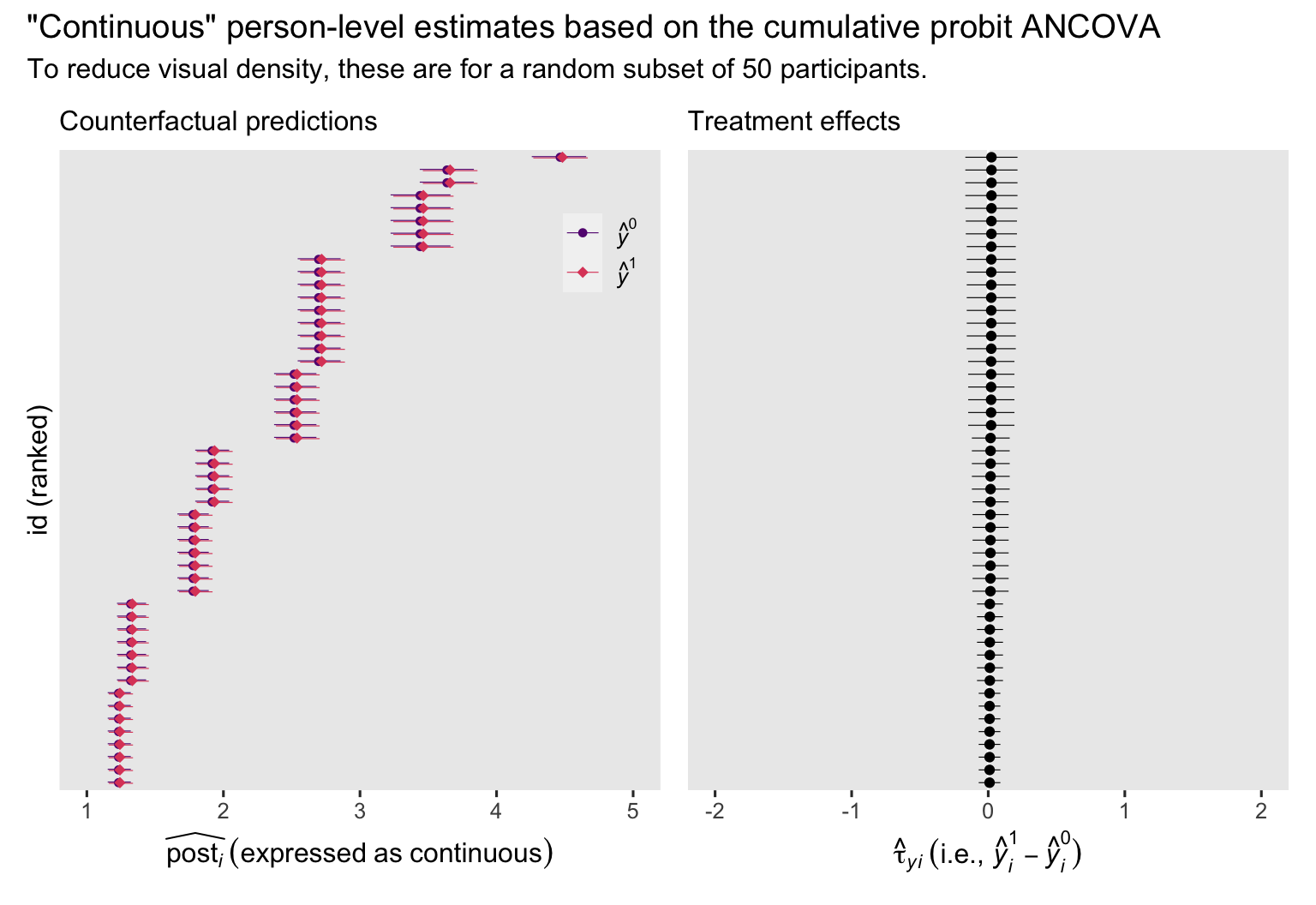
In the case of the cumulative probit ANCOVA, the \(y_i^1 - y_i^0\) contrasts do differ across participants, albeit not much in the case of the data from Coyne et al. (
2022).
Here’s how we might compute \(\tau_y^\text{ATE}\) estimate with each model.
# ANOVA
fit1_conditional_probabilities_by_id %>%
  mutate(j = as.double(.category)) %>%
  mutate(product = j * .epred) %>%
  group_by(id, protection, .draw) %>%
  summarise(y_hat = sum(product)) %>%
  pivot_wider(names_from = protection, values_from = y_hat) %>%
  # compute the protection contrast
  mutate(d = `1` - `0`) %>%
  # group and summarize across levels of id
  group_by(.draw) %>%
  summarise(d = mean(d)) %>%
  # summarize the ATE
  summarise(m = mean(d),
            s = sd(d),
            ll = quantile(d, probs = .025),
            ul = quantile(d, probs = .975))
## # A tibble: 1 × 4
##        m     s     ll    ul
##    <dbl> <dbl>  <dbl> <dbl>
## 1 0.0578 0.112 -0.165 0.276
# ANCOVA
fit2_conditional_probabilities_by_id %>%
  mutate(j = as.double(.category)) %>%
  mutate(product = j * .epred) %>%
  group_by(id, protection, .draw) %>%
  summarise(y_hat = sum(product)) %>%
  pivot_wider(names_from = protection, values_from = y_hat) %>%
  mutate(d = `1` - `0`) %>%
  group_by(.draw) %>%
  summarise(d = mean(d)) %>%
  summarise(m = mean(d),
            s = sd(d),
            ll = quantile(d, probs = .025),
            ul = quantile(d, probs = .975))
## # A tibble: 1 × 4
##        m      s     ll    ul
##    <dbl>  <dbl>  <dbl> <dbl>
## 1 0.0172 0.0714 -0.122 0.156
The poster means for the \(\tau_y^\text{ATE}\) were similar for the two models, but the posterior SD was about 40% smaller for the cumulative probit ANCOVA. Once again, baseline covaraites helped us make our causal inferences with greater precision.
\(\mathbb E (y_i^1) - \mathbb E (y_i^0)\) without and with covariates.
To use the \(\mathbb E (y_i^1) - \mathbb E (y_i^0)\) method with the cumulative probit ANOVA, we only need the simple nd predictor grid from before. Just in case you’ve forgotten, we’ll define it again. Then we’ll show the add_epred_draws()-based workflow to compute our estimates for \(\mathbb E (y_i^1)\), \(\mathbb E (y_i^1)\), and their contrast \(\tau_y^\text{ATE}\).
# we've defined this predictor grid before
nd <- tibble(protection = 0:1)

# now compute
nd %>%
  add_epred_draws(fit1) %>%
  mutate(j = as.double(.category)) %>%
  mutate(product = j * .epred) %>%
  group_by(protection, .draw) %>%
  summarise(y_hat = sum(product)) %>%
  pivot_wider(names_from = protection, values_from = y_hat) %>%
  # compute the protection contrast
  mutate(`1 - 0` = `1` - `0`) %>%
  # covert back to the long format for our conditional means and their contrast
  pivot_longer(`0`:`1 - 0`) %>%
  # group and summarize
  group_by(name) %>%
  summarise(m = mean(value),
            s = sd(value),
            ll = quantile(value, probs = .025),
            ul = quantile(value, probs = .975))
## # A tibble: 3 × 5
##   name       m      s     ll    ul
##   <chr>  <dbl>  <dbl>  <dbl> <dbl>
## 1 0     2.20   0.0763  2.05  2.35
## 2 1     2.26   0.0828  2.10  2.42
## 3 1 - 0 0.0578 0.112  -0.165 0.276
If you compare these summaries, you’ll find they’re the same values from our ANOVA-based participant-level estimates from the last section. Thus we see that when we convert the results from our cumulative probit ANOVA into a continuous-like metric,
$$ \tau_y^\text{ATE} = \mathbb E (y_i^1 - y_i^0) = \mathbb E (y_i^1) - \mathbb E (y_i^0). $$
This is not the case once we add covariates to the model. For our cumulative probit ANCOVA fit2, we can only compute \(\tau_y^\text{ATE}\) with the standardization method, as in the last section.
Just in case you were curious, here are the sample statistics for \(\bar y^0\), \(\bar y^1\), and their difference (in the case where you were willing to treat post as continuous).
coyne2022 %>%
  group_by(protection) %>%
  summarise(mean = mean(post)) %>%
  pivot_wider(names_from = protection, values_from = mean) %>%
  mutate(`1 - 0` = `1` - `0`)
## # A tibble: 1 × 3
##     `0`   `1` `1 - 0`
##   <dbl> <dbl>   <dbl>
## 1  2.19  2.25  0.0559
Thus our estimates for \(\mathbb E (y_i^1)\), \(\mathbb E (y_i^1)\), and their contrast \(\tau_y^\text{ATE}\) are very close to their sample-statistic analogues, which I find reassuring. It might not be statistically rigorous to express the results of an ordinal model in a continuous-like metric. But since we are, it’s nice to see the results resemble what we’d get if we treated the sample data as continuous, too.
Continuous-ish wrap-up.
In case it wasn’t clear, the estimands in this section are my own. I like this method because I bet many of my more applied substantive colleagues would find these estimands easy to understand, and a good effect size should make a fancy analysis easier to understand. This method is also nice in that it returns a univariate effect size, and it benefits from baseline covariates. To my eye, the method has two major limitations. First, this method is limited in that I, an non-statistician, am proposing it in a blog post. Second, this method will probably make our pals the statisticians and quantitative methodologists vomit in their mouths a little. You have to choose which crowd’s you want to speak to, friends. My goal, here, is to give y’all options.
Is this it?
No.
Try the cumulative logit.
Even though I’m a fanboy for the cumulative probit, some researchers might prefer the cumulative logit, which is the default when you set family = cumulative within the brm() function. I’ve rerun all the analyses in this blog post using that setting, and although the numeric results differ, the overall pattern of results is the same. Don’t trust me blindly, though. Try it out for yourself.
You might prefer category-specific results.
You may have missed it, but I mentioned in a footnote that brms currently allows for category-specific effects for family = cumulative models, by way of the cs() helper function. However, this functionality is experimental, so you can’t yet assume it will be there in future versions of brms (I’m currently using 2.19.0). I suspect the category-specific effects approach could be particularly interesting if you take \(\Delta_j^\text{ATE}\) as your causal estimand. But be warned: the category-specific effects approach might well come at the cost of much larger posterior SD’s.
There are other estimands.
We’ve already covered enough estimands for one blog post. But researchers have proposed other options. To learn about more, read through Boes ( 2013), Volfovsky et al. ( 2015) and Chiba ( 2018), and look through their reference sections. It’s still the Wild West in this part of the literature.
Recap
In this post, some of the main points we covered were:
- Ordinal models can make causal inference tricky. As a consequence, scholars have proposed many competing causal estimands. We covered three:
- Volfovsky et al’s
\(\tau_z^\text{ATE}\), - Boes’s
\(\Delta_y^\text{ATE}\)(what I called\(\Delta_j^\text{ATE}\), instead), and - my totally off-label
\(\tau_y^\text{ATE}\).
- Volfovsky et al’s
\(\tau_z^\text{ATE}\)is- a univariate estimand,
- expressed in terms of the underlying latent variable, which
- does NOT benefit from baseline covariates,
- is methodologically rigorous, and
- only makes sense if you like the latent-variable interpretation.
\(\Delta_y^\text{ATE}\)(aka\(\Delta_j^\text{ATE}\)) is- a multivariate estimand,
- expressed in terms of the difference in probability for each of the
\(J\)Likert response options, which - does benefit from baseline covariates,
- is methodologically rigorous, but
- may be confusing to people not obsessed with quantitative methods.
- My new
\(\tau_y^\text{ATE}\)is- a univariate estimand,
- expressed in terms of the average treatment effect after transforming the ordinal model to a continuous scale, which
- does benefit from baseline covariates,
- will probably annoy statisticians and quantitative methodologists, and
- might be more easily understood by normal humans.
- Even though we extensively explored these estimands with cumulative probit models, the overall pattern of results is the same for cumulative logit models.
Okay, I’m exhausted, which means it’s time to switch gears. In the next post, we’ll talk about change scores and how they fit into our potential outcomes causal inference framework. If you haven’t noticed, some people get up into their feelings when the conversation turns to change scores. Beware.
Thank the reviewer
I’d like to publicly acknowledge and thank
for his kind efforts reviewing the draft of this post. Go team!
Do note the final editorial decisions were my own, and I do not think it would be reasonable to assume my reviewer has given a blanket endorsement of the current version of this post.
Session info
sessionInfo()
## R version 4.3.0 (2023-04-21)
## Platform: aarch64-apple-darwin20 (64-bit)
## Running under: macOS Ventura 13.4
##
## Matrix products: default
## BLAS:   /Library/Frameworks/R.framework/Versions/4.3-arm64/Resources/lib/libRblas.0.dylib
## LAPACK: /Library/Frameworks/R.framework/Versions/4.3-arm64/Resources/lib/libRlapack.dylib;  LAPACK version 3.11.0
##
## locale:
## [1] en_US.UTF-8/en_US.UTF-8/en_US.UTF-8/C/en_US.UTF-8/en_US.UTF-8
##
## time zone: America/Chicago
## tzcode source: internal
##
## attached base packages:
## [1] stats     graphics  grDevices utils     datasets  methods   base
##
## other attached packages:
##  [1] marginaleffects_0.12.0 patchwork_1.1.2        tidybayes_3.0.4        brms_2.19.0
##  [5] Rcpp_1.0.10            lubridate_1.9.2        forcats_1.0.0          stringr_1.5.0
##  [9] dplyr_1.1.2            purrr_1.0.1            readr_2.1.4            tidyr_1.3.0
## [13] tibble_3.2.1           ggplot2_3.4.2          tidyverse_2.0.0
##
## loaded via a namespace (and not attached):
##   [1] tensorA_0.36.2       rstudioapi_0.14      jsonlite_1.8.5       magrittr_2.0.3       TH.data_1.1-2
##   [6] estimability_1.4.1   farver_2.1.1         nloptr_2.0.3         rmarkdown_2.22       vctrs_0.6.3
##  [11] minqa_1.2.5          base64enc_0.1-3      blogdown_1.17        htmltools_0.5.5      haven_2.5.2
##  [16] distributional_0.3.2 sass_0.4.6           StanHeaders_2.26.27  bslib_0.5.0          htmlwidgets_1.6.2
##  [21] plyr_1.8.8           sandwich_3.0-2       emmeans_1.8.6        zoo_1.8-12           cachem_1.0.8
##  [26] igraph_1.4.3         mime_0.12            lifecycle_1.0.3      pkgconfig_2.0.3      colourpicker_1.2.0
##  [31] Matrix_1.5-4         R6_2.5.1             fastmap_1.1.1        collapse_1.9.6       shiny_1.7.4
##  [36] digest_0.6.31        colorspace_2.1-0     ps_1.7.5             crosstalk_1.2.0      projpred_2.6.0
##  [41] labeling_0.4.2       fansi_1.0.4          timechange_0.2.0     abind_1.4-5          mgcv_1.8-42
##  [46] compiler_4.3.0       withr_2.5.0          backports_1.4.1      inline_0.3.19        shinystan_2.6.0
##  [51] gamm4_0.2-6          highr_0.10           pkgbuild_1.4.1       MASS_7.3-58.4        gtools_3.9.4
##  [56] loo_2.6.0            tools_4.3.0          httpuv_1.6.11        threejs_0.3.3        glue_1.6.2
##  [61] callr_3.7.3          nlme_3.1-162         promises_1.2.0.1     grid_4.3.0           checkmate_2.2.0
##  [66] reshape2_1.4.4       generics_0.1.3       gtable_0.3.3         tzdb_0.4.0           data.table_1.14.8
##  [71] hms_1.1.3            utf8_1.2.3           pillar_1.9.0         ggdist_3.3.0         markdown_1.7
##  [76] posterior_1.4.1      later_1.3.1          splines_4.3.0        lattice_0.21-8       survival_3.5-5
##  [81] tidyselect_1.2.0     miniUI_0.1.1.1       knitr_1.43           arrayhelpers_1.1-0   gridExtra_2.3
##  [86] bookdown_0.34        stats4_4.3.0         xfun_0.39            bridgesampling_1.1-2 matrixStats_1.0.0
##  [91] DT_0.28              rstan_2.21.8         stringi_1.7.12       yaml_2.3.7           boot_1.3-28.1
##  [96] evaluate_0.21        codetools_0.2-19     emo_0.0.0.9000       cli_3.6.1            RcppParallel_5.1.7
## [101] shinythemes_1.2.0    xtable_1.8-4         munsell_0.5.0        processx_3.8.1       jquerylib_0.1.4
## [106] coda_0.19-4          svUnit_1.0.6         parallel_4.3.0       rstantools_2.3.1     ellipsis_0.3.2
## [111] assertthat_0.2.1     prettyunits_1.1.1    dygraphs_1.1.1.6     bayesplot_1.10.0     Brobdingnag_1.2-9
## [116] lme4_1.1-33          viridisLite_0.4.2    mvtnorm_1.2-2        scales_1.2.1         xts_0.13.1
## [121] insight_0.19.2       crayon_1.5.2         rlang_1.1.1          multcomp_1.4-24      shinyjs_2.1.0
References
Boes, S. (2013). Nonparametric analysis of treatment effects in ordered response models. Empirical Economics, 44(1), 81–109. https://doi.org/10.1007/s00181-010-0354-y
Bürkner, P.-C. (2020). Bayesian item response modeling in R with brms and Stan. arXiv:1905.09501 [Stat]. http://arxiv.org/abs/1905.09501
Bürkner, P.-C. (2023). brms reference manual, Version 2.19.0. https://CRAN.R-project.org/package=brms/brms.pdf
Bürkner, P.-C., & Vuorre, M. (2019). Ordinal regression models in psychology: A tutorial. Advances in Methods and Practices in Psychological Science, 2(1), 77–101. https://doi.org/10.1177/2515245918823199
Chiba, Y. (2018). Bayesian inference of causal effects for an ordinal outcome in randomized trials. Journal of Causal Inference, 6(2). https://doi.org/10.1515/jci-2017-0019
Coyne, R., Walsh, J. C., & Noone, C. (2022). Awareness, understanding and HIV stigma in response to Undetectable=Untransmittable messages: Findings from a nationally representative sample in the united kingdom. AIDS and Behavior, 26, 3818–3826. https://doi.org/10.1007/s10461-022-03710-9
Gelman, A., Hill, J., & Vehtari, A. (2020). Regression and other stories. Cambridge University Press. https://doi.org/10.1017/9781139161879
Holland, P. W. (1986). Statistics and causal inference. Journal of the American Statistical Association, 81(396), 945–960. https://doi.org/ https://dx.doi.org/10.1080/01621459.1986.10478354
Kazdin, A. E. (2017). Research design in clinical psychology, 5th Edition. Pearson. https://www.pearson.com/
Kruschke, J. K. (2015). Doing Bayesian data analysis: A tutorial with R, JAGS, and Stan. Academic Press. https://sites.google.com/site/doingbayesiandataanalysis/
Liddell, T. M., & Kruschke, J. K. (2018). Analyzing ordinal data with metric models: What could possibly go wrong? Journal of Experimental Social Psychology, 79, 328–348. https://doi.org/10.1016/j.jesp.2018.08.009
McElreath, R. (2015). Statistical rethinking: A Bayesian course with examples in R and Stan. CRC press. https://xcelab.net/rm/statistical-rethinking/
Rubin, D. B. (1974). Estimating causal effects of treatments in randomized and nonrandomized studies. Journal of Educational Psychology, 66(5), 688–701. https://doi.org/10.1037/h0037350
Shadish, W. R., Cook, T. D., & Campbell, D. T. (2002). Experimental and quasi-experimental designs for generalized causal inference. Houghton, Mifflin and Company.
Solomon, R. L. (1949). An extension of control group design. Psychological Bulletin, 46(2), 137–150. https://doi.org/10.1037/h0062958
Volfovsky, A., Airoldi, E. M., & Rubin, D. B. (2015). Causal inference for ordinal outcomes. arXiv. https://doi.org/10.48550/arXiv.1501.01234
-
Word on the street is all the cool kids are using feelings integers, these days. ↩︎
-
No, I did not just name this study design after myself. The Solomon four-group design comes from the late psychologist Richard L. Solomon, who proposed the design in a ( 1949) paper. In short, the Solomon four-group design allows researchers to measure the degree to which pretesting might influence the results of an intervention. Say you have two interventions: treatment and control. The Solomon four-group is effectively two experiments in one, one of which is a pre-post RCT, and the other is a post-assessment-only RCT. Since we’ll only be focusing on the pre-post RCT part of Coyne et al’s data, I really don’t want to get caught up in the nuances of the study design. But if you want to learn more, read Solomon’s original ( 1949) paper. The Solomon four-group was also briefly covered in Shadish et al. ( 2002), and more fully explored in Kazdin ( 2017). ↩︎
-
The full data set has other interesting baseline covariates.
Sexuality, for example, might seem methodologically and substantively interesting to consider in these analyses. But frankly, two baseline covariates will be more than enough for our purposes. Feel free to play around with other items from the full data set on your own, though. ↩︎ -
If you’re disturbed by how imperfectly the models captured the sample data, consider fitting models with category-specific effects. This is currently allowed for
family = cumulative(probit)models as an experimental feature of thecs()function. You can learn more aboutcs()in the Special predictor terms subsection of thebrmsformulasection of the brms reference manual ( Bürkner, 2023). ↩︎ -
In some parts of the literature, the ordinal variable is termed
\(Y\)and the continuous underlying latent variable is termed\(Y^*\). However, Volfovsky et al. ( 2015) favored the\(Z\)notation. Plus, nobody in their right mind would want to write out\(\tau_{y^*}^\text{ATE}\)for their causal estimand. ↩︎ -
We saw that Gaussian and gamma model have this convenience, but only when one uses the identity link. For a refresher, see the last post. ↩︎
-
😭 ↩︎
-
You, of course, are free to care about the CATE in your own work. During this period of my professional development, I’m all about that ATE. ↩︎
- Posted on:
- May 21, 2023
- Length:
- 66 minute read, 13851 words