Causal inference with Bayesian models

In the first two posts of this series, we relied on ordinary least squares (OLS). In the third post, we expanded to maximum likelihood for a couple logistic regression models. In all cases, we approached inference from a frequentist perspective. In this fourth post, we’re finally ready to make causal inferences as Bayesians. We’ll do so by refitting the Gaussian and binomial models from the previous posts with the Bayesian brms package ( Bürkner, 2017, 2018, 2022), and show how to compute our primary estimates, such as the ATE, when working with posterior draws. Along the way, we will also discuss different approaches to priors, and practice writing the Bayesian models with formal statistical notation.

Compared to the others, this post will be very light on theory, and heavy on methods. So if you don’t love that Bayes, you can feel free to skip this one. I should also clarify that if you are a new Bayesian, or are unfamiliar with the brms package, this is not the post for you. I will be assuming my readers have basic fluency with both throughout. If you need to firm up your foundations, check out the resources listed here.

Gaussian models as a Bayesian

Let’s revisit the Horan & Johnson ( 1971) data from the first two posts.

# load packages
library(tidyverse)
library(brms)
library(tidybayes)
library(marginaleffects)

# adjust the global theme
theme_set(theme_gray(base_size = 13) +
            theme(panel.grid = element_blank()))

# load the data from GitHub
load(url("https://github.com/ASKurz/blogdown/raw/main/content/blog/2023-04-12-boost-your-power-with-baseline-covariates/data/horan1971.rda?raw=true"))

# wrangle a bit
horan1971 <- horan1971 %>% 
  filter(treatment %in% c("delayed", "experimental")) %>% 
  mutate(prec = pre - mean(pre),
         experimental = ifelse(treatment == "experimental", 1, 0))

Now we’ve got our data, we’re ready to fit some Bayesian models.

Gaussian models.

Instead of expressing our models in OLS-style notation where we include \(\epsilon_i\), it’s time we switch to the Gaussian likelihoodist format. Here’s what our Gaussian ANOVA-type model might look like when including Bayesian priors:

$$ \begin{align*} \text{post}_i & \sim \operatorname{Normal}(\mu_i, \sigma) \\ \mu_i & = \beta_0 + \beta_1 \text{experimental}_i \\ \beta_0 & \sim \operatorname{Normal}(156.5, 15) \\ \beta_1 & \sim \operatorname{Normal}(0, 15) \\ \sigma & \sim \operatorname{Exponential}(0.067). \end{align*} $$

The prior for \(\beta_0\) is centered on 156.5 because according to the Centers for Disease Control and Prevention (CDC; see here), that is the average weight for 19-year-old women in the US in recent years (2015-2018). Granted, the Horan & Johnson ( 1971) data were from more than 50 years ago, but since body weight has increased over the past few decades in the US, an average woman’s weight now might be a decent first approximation for a woman considered overweight at that time. The standard deviation of 15 in the prior is meant to reflect uncertainty, and it suggests we think about 95% of the prior mass should be between 30 points below and above the prior mean.

The prior for \(\beta_1\) is centered on 0 to weakly regularize the estimate for the experimental difference towards smaller values. However, we continue to use a fairly permissive standard deviation of 15 to allow for somewhat large treatment effects. That is, there could be a difference between the groups as large as 30 pounds either way, but smaller differences are more plausible than larger ones.

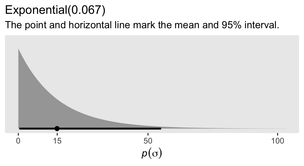
When switching to the likelihoodist framework, we speak in terms of \(\sigma\), rather than \(\epsilon\). Since \(\sigma\) must be positive, we have used the exponential distribution for the prior.¹ The exponential distribution has a single parameter, \(\lambda\), which is the reciprocal of the mean.² Though I’m no weight or weight-loss researcher, my first blind guess at a standard deviation for women’s weights is somewhere around 15, which we can express by setting the rate to about 0.067.

1 / 15  # the exponential rate is the reciprocal of the mean

## [1] 0.06666667

If you haven’t worked with exponential priors for \(\sigma\) parameters before, they’re nice in that they place a lot of uncertainty around the mean. To give you a sense, here’s what our \(\operatorname{Exponential}(0.067)\) prior looks like in a plot.

prior(exponential(0.067), class = sd) %>% 
  parse_dist() %>% 
  
  ggplot(aes(y = 0, dist = .dist, args = .args)) +
  stat_halfeye(point_interval = mean_qi, .width = .95) +
  scale_x_continuous(expression(italic(p)(sigma)), breaks = c(0, 15, 50, 100)) +
  scale_y_continuous(NULL, breaks = NULL) +
  labs(title = "Exponential(0.067)",
       subtitle = "The point and horizontal line mark the mean and 95% interval.")

Extrapolating, we might express our Bayesian Gaussian ANCOVA-type model as

$$ \begin{align*} \text{post}_i & \sim \operatorname{Normal}(\mu_i, \sigma) \\ \mu_i & = \beta_0 + \beta_1 \text{experimental}_i + \beta_2 \text{prec}_i\\ \beta_0 & \sim \operatorname{Normal}(156.5, 15) \\ \beta_1 & \sim \operatorname{Normal}(0, 15) \\ \beta_2 & \sim \operatorname{Normal}(0.75, 0.25) \\ \sigma & \sim \operatorname{Exponential}(0.133), \end{align*} $$

where the new parameter \(\beta_2\) accounts for our baseline covariate, the mean-centered weights before the intervention (prec). For simplicity, the priors for \(\beta_0\) and \(\beta_1\) are the same as before.

The prior for our new parameter \(\beta_2\) is more certain than the others. This is because, even as someone who does not do weight-loss research, I am very confident that a variable like weight will have a strong positive correlation before and after an 8-week period.³ Thus we should expect \(\beta_2\) to be somewhere between about 0.5 and 1. Here’s what the \(\operatorname{Normal}(0.75, 0.25)\) prior looks like:

prior(normal(0.75, 0.25), class = sd) %>% 
  parse_dist() %>% 
  
  ggplot(aes(y = 0, dist = .dist, args = .args)) +
  stat_halfeye(point_interval = mean_qi, .width = .95,
               p_limits = c(.0001, .9999)) +
  scale_y_continuous(NULL, breaks = NULL) +
  coord_cartesian(xlim = c(0, 1.5)) +
  labs(title = "Normal(0.75, 0.25)",
       subtitle = "The point and horizontal line mark the mean and 95% interval.",
       x = expression(italic(p)(beta[2])))

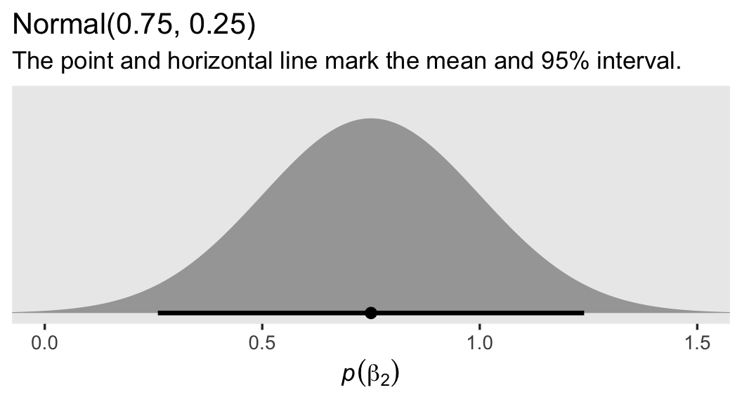
Frankly, I think you could even justify a tighter prior than this. As to \(\sigma\), I’m now using an exponential distribution with a mean of 7.5, which is half the magnitude we used in the previous model. This is to account for the substantial amount of variation I expect to account for with our high-quality baseline covariate prec.

1 / 7.5  # the exponential rate is the reciprocal of the mean

## [1] 0.1333333

My guess is a proper weight-loss researcher could come up with better priors, but I’m comfortable using these for the sake of a blog. Here’s how to fit these two models with the brm() function from the brms package. Note our use of the seed argument, which makes the results more reproducible.

# Bayesian Gaussian ANOVA
fit1 <- brm(
  data = horan1971,
  family = gaussian,
  post ~ 0 + Intercept + experimental,
  prior = prior(normal(156.5, 15), class = b, coef = Intercept) +
    prior(normal(0, 15), class = b, coef = experimental) +
    prior(exponential(0.067), class = sigma),
  cores = 4, seed = 4
)

# Bayesian Gaussian ANCOVA
fit2 <- brm(
  data = horan1971,
  family = gaussian,
  post ~ 0 + Intercept + experimental + prec,
  prior = prior(normal(156.5, 15), class = b, coef = Intercept) +
    prior(normal(0, 15), class = b, coef = experimental) +
    prior(normal(0.75, 0.25), class = b, coef = prec) +
    prior(exponential(0.133), class = sigma),
  cores = 4, seed = 4
)

For brms users not used to the 0 + Intercept syntax, read through my discussions here or here, and study the set_prior and brmsformula sections of the brms reference manual ( Bürkner, 2023). In short, if you have not mean-centered all of your predictor variables, you might should use the 0 + Intercept syntax. In our case, the prec is mean centered, but the experimental dummy is not, so 0 + Intercept syntax is my syntax of choice.

In this case, the parameter summaries for these two models are pretty close to their OLS analogues from earlier posts. We can view them with either the print() or summary() functions.

print(fit1)

##  Family: gaussian 
##   Links: mu = identity; sigma = identity 
## Formula: post ~ 0 + Intercept + experimental 
##    Data: horan1971 (Number of observations: 41) 
##   Draws: 4 chains, each with iter = 2000; warmup = 1000; thin = 1;
##          total post-warmup draws = 4000
## 
## Population-Level Effects: 
##              Estimate Est.Error l-95% CI u-95% CI Rhat Bulk_ESS Tail_ESS
## Intercept      153.97      3.61   147.22   161.25 1.00     2062     1858
## experimental    -2.39      5.11   -12.41     7.63 1.00     2023     2153
## 
## Family Specific Parameters: 
##       Estimate Est.Error l-95% CI u-95% CI Rhat Bulk_ESS Tail_ESS
## sigma    17.53      2.01    14.13    21.97 1.00     2496     2435
## 
## Draws were sampled using sampling(NUTS). For each parameter, Bulk_ESS
## and Tail_ESS are effective sample size measures, and Rhat is the potential
## scale reduction factor on split chains (at convergence, Rhat = 1).

print(fit2)

##  Family: gaussian 
##   Links: mu = identity; sigma = identity 
## Formula: post ~ 0 + Intercept + experimental + prec 
##    Data: horan1971 (Number of observations: 41) 
##   Draws: 4 chains, each with iter = 2000; warmup = 1000; thin = 1;
##          total post-warmup draws = 4000
## 
## Population-Level Effects: 
##              Estimate Est.Error l-95% CI u-95% CI Rhat Bulk_ESS Tail_ESS
## Intercept      154.77      1.43   151.86   157.52 1.00     3079     2565
## experimental    -4.52      2.07    -8.60    -0.40 1.00     3057     2732
## prec             0.90      0.06     0.78     1.02 1.00     3301     2560
## 
## Family Specific Parameters: 
##       Estimate Est.Error l-95% CI u-95% CI Rhat Bulk_ESS Tail_ESS
## sigma     6.55      0.78     5.25     8.20 1.00     3215     2461
## 
## Draws were sampled using sampling(NUTS). For each parameter, Bulk_ESS
## and Tail_ESS are effective sample size measures, and Rhat is the potential
## scale reduction factor on split chains (at convergence, Rhat = 1).

Counterfactual interventions, no covariates, with the Gauss.

Conceptually, our primary estimand \(\tau_\text{ATE}\) is the same for Bayesians as it is for frequentists, in that

$$\tau_\text{ATE} = \mathbb E (y_i^1 - y_i^0) = \mathbb E (y_i^1) - \mathbb E (y_i^0).$$

So all the equations we learned about in the last couple posts remain valid. However, applied Bayesian inference via MCMC methods adds a new procedural complication for the \(\mathbb E (y_i^1 - y_i^0)\) method. If you let \(j\) stand for a given MCMC draw, we end up computing

$$\tau_{\text{ATE}_j} = \mathbb E_j (y_{ij}^1 - y_{ij}^0), \ \text{for}\ j = 1, \dots, J,$$

which in words means we compute the familiar \(\mathbb E (y_i^1 - y_i^0)\) for each of the \(J\) MCMC draws. This returns a \(J\)-row vector for the \(\tau_\text{ATE}\) distribution, which we can then summarize the same as we would any other dimension of the posterior distribution. You’ll see. Anyway, the workflow in this section will follow the same basic order we used in the second post. Let’s get to work!

Compute \(\mathbb E (y_i^1) - \mathbb E (y_i^0)\) from fit1.

Before we go into full computation mode, we might want to streamline some of our summarizing code with a custom function. Many of the functions from the brms package summarize the posterior draws in terms of their mean, standard deviation, and percentile-based 95% intervals. Those, recall, are common Bayesian analogues to the frequentist point estimate, standard error, and 95% confidence intervals, respectively. Here we’ll make a custom function that will compute those summary statistics for all vectors in a data frame.

brms_summary <- function(x) {
  posterior::summarise_draws(x, "mean", "sd",  ~quantile(.x, probs = c(0.025, 0.975)))
}

To give credit where it’s due, the internals for our brms_summary() function come from the posterior package ( Bürkner et al., 2022). To give you a sense of how this works, here’s how to use brms_summary() for the three model parameters from our Bayesian ANOVA fit1.

# retrieve the MCMC draws
as_draws_df(fit1) %>% 
  # subset to our 3 focal columns
  select(b_Intercept:sigma) %>% 
  # summarize
  brms_summary()

## # A tibble: 3 × 5
##   variable         mean    sd `2.5%` `97.5%`
##   <chr>           <num> <num>  <num>   <num>
## 1 b_Intercept    154.    3.61  147.   161.  
## 2 b_experimental  -2.39  5.11  -12.4    7.63
## 3 sigma           17.5   2.01   14.1   22.0

Now we have brms_summary(), and we’re all warmed up, it’s time to compute the ATE via the \(\mathbb E (y_i^1) - \mathbb E (y_i^0)\) method. As our first attempt, we’ll use a fitted()-based approach.

# define the predictor grid
nd <- tibble(experimental = 0:1)

# compute
fitted(fit1,
       newdata = nd,
       summary = F) %>% 
  # wrangle
  data.frame() %>% 
  set_names(pull(nd, experimental)) %>% 
  mutate(ate = `1` - `0`) %>% 
  # summarize!
  brms_summary()

## # A tibble: 3 × 5
##   variable   mean    sd `2.5%` `97.5%`
##   <chr>     <num> <num>  <num>   <num>
## 1 0        154.    3.61  147.   161.  
## 2 1        152.    3.86  144.   159.  
## 3 ate       -2.39  5.11  -12.4    7.63

The first two rows of the output are the posterior summaries for \(\mathbb E (y_i^0)\) and \(\mathbb E (y_i^1)\), and the final row is the summary for our focal estimate \(\tau_\text{ATE}\).

Many of the functions from the marginaleffects package will work with brms models, too. For example, here’s the same kind of predictions()-based workflow we used in the last two blog posts, but now applied to our Bayesian ANOVA.

# predicted means
predictions(fit1, newdata = nd, by = "experimental")

## 
##  experimental Estimate 2.5 % 97.5 %
##             0      154   147    161
##             1      152   144    159
## 
## Columns: rowid, experimental, estimate, conf.low, conf.high, post

# ATE
predictions(fit1, newdata = nd, by = "experimental", hypothesis = "revpairwise")

## 
##   Term Estimate 2.5 % 97.5 %
##  1 - 0    -2.29 -12.4   7.63
## 
## Columns: term, estimate, conf.low, conf.high

In Arel-Bundock’s ( 2023) vignette, Bayesian analysis with brms, we learn the marginaleffects package defaults to summarizing Bayesian posteriors by their medians. But I generally prefer the brms convention of summarizing them by their means. If you’d like to change the marginaleffects default to use the mean, too, you can execute the following.

options(marginaleffects_posterior_center = mean)

The change in the output is subtle. The column labels all look the same, but the summary statistics in the Estimate column is now the mean, rather than the median.

# predicted means
predictions(fit1, newdata = nd, by = "experimental")

## 
##  experimental Estimate 2.5 % 97.5 %
##             0      154   147    161
##             1      152   144    159
## 
## Columns: rowid, experimental, estimate, conf.low, conf.high, post

# ATE
predictions(fit1, newdata = nd, by = "experimental", hypothesis = "revpairwise")

## 
##   Term Estimate 2.5 % 97.5 %
##  1 - 0    -2.39 -12.4   7.63
## 
## Columns: term, estimate, conf.low, conf.high

These results are now exactly the same as the ones we computed by hand with the fitted()-based code, above. If desired, you could change the settings back to the default by executing options(marginaleffects_posterior_center = stats::median). As for me, I’m going to continue using the posterior mean for the rest of this blog post.

Compute \(\mathbb E (y_i^1 - y_i^0)\) from fit1.

Before we compute our Bayesian posterior estimate for the ATE with the \(\mathbb E (y_i^1 - y_i^0)\) method, we’ll first need to redefine our predictor grid nd.

nd <- horan1971 %>% 
  select(sn) %>% 
  expand_grid(experimental = 0:1) %>% 
  mutate(row = 1:n())

# what?
glimpse(nd)

## Rows: 82
## Columns: 3
## $ sn           <int> 1, 1, 2, 2, 3, 3, 4, 4, 5, 5, 6, 6, 7, 7, 8, 8, 9, 9, 10, 10, 11, 11, 12, 12, 13, 13, 14, 14, 15,…
## $ experimental <int> 0, 1, 0, 1, 0, 1, 0, 1, 0, 1, 0, 1, 0, 1, 0, 1, 0, 1, 0, 1, 0, 1, 0, 1, 0, 1, 0, 1, 0, 1, 0, 1, 0…
## $ row          <int> 1, 2, 3, 4, 5, 6, 7, 8, 9, 10, 11, 12, 13, 14, 15, 16, 17, 18, 19, 20, 21, 22, 23, 24, 25, 26, 27…

Notice that unlike what we’ve done before, we added a row index. This will help us join our nd data to the fitted() output, below. Speaking of which, here’s how we might compute the posterior summaries for the ATE. Since this is a long block of code, I’ll provide more annotation than usual.

# compute the posterior predictions
fitted(fit1,
       newdata = nd,
       summary = F) %>% 
  # convert the results to a data frame
  data.frame() %>% 
  # rename the columns
  set_names(pull(nd, row)) %>% 
  # add a numeric index for the MCMC draws
  mutate(draw = 1:n()) %>% 
  # convert to the long format
  pivot_longer(-draw) %>% 
  # convert the row column from the character format to the numeric format
  mutate(row = as.double(name)) %>% 
  # join the nd predictor grid to the output
  left_join(nd, by = "row") %>% 
  # drop two of the columns which are now unnecessary
  select(-name, -row) %>% 
  # convert to a wider format so we can compute the contrast
  pivot_wider(names_from = experimental, values_from = value) %>% 
  # compute the ATE contrast
  mutate(tau = `1` - `0`) %>% 
  # compute the average ATE value within each MCMC draw
  group_by(draw) %>% 
  summarise(ate = mean(tau)) %>% 
  # remove the draw index column
  select(ate) %>% 
  # now summarize the ATE across the MCMC draws
  brms_summary()

## # A tibble: 1 × 5
##   variable  mean    sd `2.5%` `97.5%`
##   <chr>    <num> <num>  <num>   <num>
## 1 ate      -2.39  5.11  -12.4    7.63

Returning to the equation from a two sections up, the group_by() and summarise() lines were how we computed \(\mathbb E_j (y_{ij}^1 - y_{ij}^0)\) for each of the \(J\) MCMC draws. It was then in the final brms_summary() line where we summarized the vector of all those resulting \(\tau_{\text{ATE}_j}\) results. If you’re confused by why we included the group_by() and summarise() lines before the final summary, I was too at first. It turns out that for the Gaussian and/or ANOVA models, those intermediary steps are not necessary. However, they are necessary for non-Gaussian ANCOVA models. So my recommendation is you just get into the habit of this approach. If you’d like more on the topic, check out Section 19.4 from Gelman et al. ( 2020).

We can make the same computation with the marginaleffects::avg_comparisons() function.

avg_comparisons(fit1, variables = "experimental")

## 
##          Term Contrast Estimate 2.5 % 97.5 %
##  experimental    1 - 0    -2.39 -12.4   7.63
## 
## Columns: term, contrast, estimate, conf.low, conf.high

Not only are the results from the fitted()- and avg_comparisons()-based approaches identical, here, but they’re also identical to the results from the previous section. Which method is better? Well, the avg_comparisons() is very thrifty and convenient, which is great if you know what you’re doing. The fitted() approach is long and cumbersome, but you can keep track of exactly what’s happening at each step of the progression, which is great for learning. You get to choose which method suits your purposes best.

Counterfactual interventions, with covariates, with the Gauss.

Compute \(\mathbb E (y_i^1 \mid \bar c) - \mathbb E (y_i^0 \mid \bar c)\) from fit2.

Before we can use the \(\mathbb E (y_i^1 \mid \bar c) - \mathbb E (y_i^0 \mid \bar c)\) method, we need to redefine our nd predictor grid, which now includes the mean of prec.

nd <- horan1971 %>% 
  summarise(prec = mean(prec)) %>% 
  expand_grid(experimental = 0:1)

# what?
print(nd)

## # A tibble: 2 × 2
##        prec experimental
##       <dbl>        <int>
## 1 -8.67e-15            0
## 2 -8.67e-15            1

For our Bayesian ANCOVA, the fitted()-based workflow is much the same as for the ANOVA in the previous section. After the basic computation, we convert the output to a data fame, rename the columns, use simple subtraction to compute an ate column, and then finally summarize as desired.

fitted(fit2,
       newdata = nd,
       summary = F) %>% 
  data.frame() %>% 
  set_names(pull(nd, experimental)) %>% 
  mutate(ate = `1` - `0`) %>% 
  brms_summary()

## # A tibble: 3 × 5
##   variable   mean    sd `2.5%` `97.5%`
##   <chr>     <num> <num>  <num>   <num>
## 1 0        155.    1.43 152.   158.   
## 2 1        150.    1.53 147.   153.   
## 3 ate       -4.52  2.07  -8.60  -0.402

The thrifty predictions() version of the code remains much the same as before, too.

# predicted means
predictions(fit2, newdata = nd, by = "experimental")

## 
##  experimental Estimate 2.5 % 97.5 %      prec
##             0      155   152    158 -8.67e-15
##             1      150   147    153 -8.67e-15
## 
## Columns: rowid, experimental, estimate, conf.low, conf.high, prec, post

# ATE
predictions(fit2, newdata = nd, by = "experimental", hypothesis = "revpairwise")

## 
##   Term Estimate 2.5 % 97.5 %
##  1 - 0    -4.52  -8.6 -0.402
## 
## Columns: term, estimate, conf.low, conf.high

Happily, the results are the same whether you use a fitted()- or predictions()-based workflow. One workflow is explicit, but requires many more lines. The other workflow is more opaque, but very convenient. Everyone’s happy; we all can eat cake.

Compute \(\mathbb E (y_i^1 - y_i^0 \mid c_i)\) from fit2.

To prepare for the \(\mathbb E (y_i^1 - y_i^0 \mid c_i)\) method, we need to redefine the nd predictor grid, which once again includes a row index.

nd <- horan1971 %>% 
  select(sn, prec) %>% 
  expand_grid(experimental = 0:1) %>% 
  mutate(row = 1:n())

# what?
glimpse(nd)

## Rows: 82
## Columns: 4
## $ sn           <int> 1, 1, 2, 2, 3, 3, 4, 4, 5, 5, 6, 6, 7, 7, 8, 8, 9, 9, 10, 10, 11, 11, 12, 12, 13, 13, 14, 14, 15,…
## $ prec         <dbl> -5.335366, -5.335366, -23.585366, -23.585366, -8.335366, -8.335366, -21.585366, -21.585366, -23.8…
## $ experimental <int> 0, 1, 0, 1, 0, 1, 0, 1, 0, 1, 0, 1, 0, 1, 0, 1, 0, 1, 0, 1, 0, 1, 0, 1, 0, 1, 0, 1, 0, 1, 0, 1, 0…
## $ row          <int> 1, 2, 3, 4, 5, 6, 7, 8, 9, 10, 11, 12, 13, 14, 15, 16, 17, 18, 19, 20, 21, 22, 23, 24, 25, 26, 27…

Now compute the posterior summary for the ATE via the \(\mathbb E (y_i^1 - y_i^0 \mid c_i)\) method based on the MCMC draws from our Bayesian ANCOVA fit2.

fitted(fit2,
       newdata = nd,
       summary = F) %>% 
  data.frame() %>% 
  set_names(pull(nd, row)) %>% 
  mutate(draw = 1:n()) %>% 
  pivot_longer(-draw) %>% 
  mutate(row = as.double(name)) %>% 
  left_join(nd, by = "row") %>% 
  select(-name, -row) %>% 
  pivot_wider(names_from = experimental, values_from = value) %>% 
  mutate(tau = `1` - `0`) %>% 
  # first compute the ATE within each MCMC draw
  group_by(draw) %>% 
  summarise(ate = mean(tau)) %>% 
  select(ate) %>% 
  # now summarize the ATE across the MCMC draws
  brms_summary()

## # A tibble: 1 × 5
##   variable  mean    sd `2.5%` `97.5%`
##   <chr>    <num> <num>  <num>   <num>
## 1 ate      -4.52  2.07  -8.60  -0.402

Now confirm it works with the avg_comparisons() approach.

avg_comparisons(fit2, variables = "experimental")

## 
##          Term Contrast Estimate 2.5 % 97.5 %
##  experimental    1 - 0    -4.52  -8.6 -0.402
## 
## Columns: term, contrast, estimate, conf.low, conf.high

Whether using a fitted()- or avg_comparisons()-based workflow, the results are identical to the posterior summary for the \(\beta_1\) parameter.

# retrieve the MCMC draws
as_draws_df(fit2) %>% 
  # subset to our 3 focal columns
  transmute(`beta[1]` = b_experimental) %>% 
  # summarize
  brms_summary()

## # A tibble: 1 × 5
##   variable  mean    sd `2.5%` `97.5%`
##   <chr>    <num> <num>  <num>   <num>
## 1 beta[1]  -4.52  2.07  -8.60  -0.402

Just as we learned with the earlier frequentist analyses of these data, the \(\beta_1\) parameter is the same as the ATE when using the Gaussian likelihood with the conventional identity link. This convenient property, however, will not extend to other contexts. Speaking of which, let’s go logistic.

Logistic regression

For the second half of this post, let’s revisit the Wilson et al. ( 2017) data from the last post. Here we load the data, subset, and wrangle them just like before.

wilson2017 <- readxl::read_excel("data/pmed.1002479.s001.xls", sheet = "data")

# subset
set.seed(1)

wilson2017 <- wilson2017 %>% 
  mutate(msm = ifelse(msm == 99, NA, msm)) %>% 
  drop_na(anytest, gender, partners, msm, ethnicgrp, age) %>% 
  slice_sample(n = 400) %>% 
  # factors
  mutate(gender    = factor(gender, levels = c("Female", "Male")),
         msm       = factor(msm, levels = c("other", "msm")),
         partners  = factor(partners, levels = c(1:9, "10+")),
         ethnicgrp = factor(ethnicgrp,
                            levels = c("White/ White British", "Asian/ Asian British", "Black/ Black British", "Mixed/ Multiple ethnicity", "Other"))) %>% 
  # z-score
  mutate(agez = (age - mean(age)) / sd(age)) %>% 
  # make a simple treatment dummy
  mutate(tx = ifelse(group == "SH:24", 1, 0)) %>% 
  rename(id = anon_id) %>% 
  select(id, tx, anytest, gender, partners, msm, ethnicgrp, age, agez)

# what?
glimpse(wilson2017)

## Rows: 400
## Columns: 9
## $ id        <dbl> 20766, 18778, 15678, 20253, 23805, 17549, 16627, 16485, 21905, 22618, 18322, 22481, 23708, 16817, 24…
## $ tx        <dbl> 0, 1, 0, 1, 0, 0, 1, 0, 0, 1, 1, 1, 1, 1, 1, 0, 0, 1, 0, 1, 1, 1, 1, 0, 1, 1, 1, 1, 0, 0, 0, 0, 0, 0…
## $ anytest   <dbl> 0, 0, 0, 1, 1, 0, 0, 0, 0, 1, 0, 1, 0, 0, 1, 1, 0, 1, 0, 0, 0, 1, 0, 1, 1, 1, 0, 0, 0, 0, 1, 1, 0, 0…
## $ gender    <fct> Male, Male, Female, Male, Female, Female, Male, Female, Male, Male, Female, Female, Male, Female, Fe…
## $ partners  <fct> 2, 4, 2, 1, 4, 2, 1, 2, 10+, 1, 1, 1, 1, 1, 2, 10+, 4, 10+, 1, 3, 1, 1, 1, 2, 3, 4, 3, 10+, 1, 1, 3,…
## $ msm       <fct> other, other, other, other, other, other, other, other, other, other, other, other, other, other, ot…
## $ ethnicgrp <fct> White/ White British, White/ White British, Mixed/ Multiple ethnicity, White/ White British, White/ …
## $ age       <dbl> 21, 19, 17, 20, 24, 19, 18, 20, 29, 28, 20, 23, 24, 24, 24, 20, 19, 27, 17, 23, 25, 23, 24, 19, 24, …
## $ agez      <dbl> -0.53290527, -1.10362042, -1.67433557, -0.81826284, 0.32316745, -1.10362042, -1.38897799, -0.8182628…

Even though the full data set has responses from more than 2,000 people, the \(n = 400\) subset is plenty for our purposes.

Binomial models.

Here’s what the binomial⁴ ANOVA-type model for the anytest variable might look like when including our Bayesian priors:

$$ \begin{align*} \text{anytest}_i & \sim \operatorname{Binomial}(n = 1, p_i) \\ \operatorname{logit}(p_i) & = \beta_0 + \beta_1 \text{tx}_i \\ \beta_0 & \sim \operatorname{Normal}(0, 1.25) \\ \beta_1 & \sim \operatorname{Normal}(0, 1). \end{align*} $$

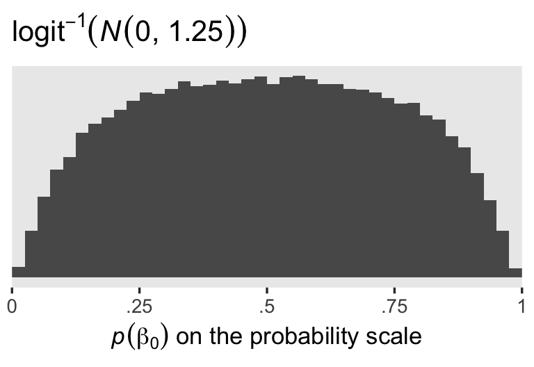
Since I’m not a medical researcher, I’m switching to a more generic weakly-regularizing approach to the priors for this model and the next. When you’re using the conventional logit link, the \(\operatorname{Normal}(0, 1.25)\) prior will gently nudge the \(\beta_0\) posterior toward the middle of the probability space, while allowing for estimates anywhere along the possible range. To give you a sense, here are 100,000 draws from \(\operatorname{Normal}(0, 1.25)\), which are then converted back to the probability space with the inverse logit function.

set.seed(4)
tibble(n = rnorm(n = 1e5, mean = 0, sd = 1.25)) %>% 
  mutate(p = inv_logit_scaled(n)) %>% 
  ggplot(aes(p)) +
  geom_histogram(boundary = 0, binwidth = 0.025) +
  scale_x_continuous(labels = c("0", ".25", ".5", ".75", "1"), expand = c(0, 0)) +
  scale_y_continuous(NULL, breaks = NULL) +
  labs(title = expression(logit^{-1}*(italic(N)(0*", "*1.25))),
       x = expression(italic(p)(beta[0])*" on the probability scale"))

The \(\operatorname{Normal}(0, 1)\) prior for the active treatment coefficient, \(\beta_1\), is also a generic weakly-regularizing prior on the logit scale.

Now here’s the formula for the Bayesian ANCOVA version of the model:

$$ \begin{align*} \text{anytest}_i & \sim \operatorname{Binomial}(n = 1, p_i) \\ \operatorname{logit}(p_i) & = \beta_0 + \beta_1 \text{tx}_i \\ & \;\; + \beta_2 \text{agez}_i \\ & \;\; + \beta_3 \text{Male}_i \\ & \;\; + \beta_4 \text{MSM}_i \\ & \;\; + \beta_5 \text{Asian}_i + \beta_6 \text{Black}_i + \beta_7 \text{Mixed}_i + \beta_8 \text{Other}_i \\ & \;\; + \beta_9 \text{partners2}_i + \beta_{10} \text{partners3}_i + \dots + \beta_{17} \text{partners10}\texttt{+}_i \\ \beta_0 & \sim \operatorname{Normal}(0, 1.25) \\ \beta_1, \dots, \beta_{17} & \sim \operatorname{Normal}(0, 1). \end{align*} $$

For simplicity, we’re extending the generic \(\operatorname{Normal}(0, 1)\) prior to all predictor variables in the ANCOVA version of the model. I have no doubt a real medical researcher could have set better priors. This is what you get when you let a psychologist put his mitts on your data.

Here’s how to fit the Bayesian binomial models with the brm() function.

# Bayesian binomial ANOVA
fit3 <- brm(
  data = wilson2017,
  family = binomial,
  anytest | trials(1) ~ 0 + Intercept + tx,
  prior = prior(normal(0, 1.25), class = b, coef = Intercept) +
    prior(normal(0, 1), class = b, coef = tx),
  cores = 4, seed = 4
)

# Bayesian binomial ANCOVA
fit4 <- brm(
  data = wilson2017,
  family = binomial,
  anytest | trials(1) ~ 0 + Intercept + tx + agez + gender + msm + ethnicgrp + partners,
  prior = prior(normal(1, 1.25), class = b, coef = Intercept) +
    prior(normal(0, 1), class = b),
  cores = 4, seed = 4
)

The parameter summary for the binomial ANCOVA fit3 is pretty similar to the results from the glm()-based version of the model. You’ll note many of the parameters from our Bayesian fit4 are more conservative compared to its frequentist counterpart. That’s what happens when you use regularizing priors.

print(fit3)

##  Family: binomial 
##   Links: mu = logit 
## Formula: anytest | trials(1) ~ 0 + Intercept + tx 
##    Data: wilson2017 (Number of observations: 400) 
##   Draws: 4 chains, each with iter = 2000; warmup = 1000; thin = 1;
##          total post-warmup draws = 4000
## 
## Population-Level Effects: 
##           Estimate Est.Error l-95% CI u-95% CI Rhat Bulk_ESS Tail_ESS
## Intercept    -1.11      0.16    -1.44    -0.80 1.00     1387     1786
## tx            0.81      0.21     0.39     1.22 1.00     1372     1713
## 
## Draws were sampled using sampling(NUTS). For each parameter, Bulk_ESS
## and Tail_ESS are effective sample size measures, and Rhat is the potential
## scale reduction factor on split chains (at convergence, Rhat = 1).

print(fit4)

##  Family: binomial 
##   Links: mu = logit 
## Formula: anytest | trials(1) ~ 0 + Intercept + tx + agez + gender + msm + ethnicgrp + partners 
##    Data: wilson2017 (Number of observations: 400) 
##   Draws: 4 chains, each with iter = 2000; warmup = 1000; thin = 1;
##          total post-warmup draws = 4000
## 
## Population-Level Effects: 
##                                  Estimate Est.Error l-95% CI u-95% CI Rhat Bulk_ESS Tail_ESS
## Intercept                           -1.11      0.25    -1.60    -0.63 1.00     3395     3130
## tx                                   0.92      0.23     0.48     1.36 1.00     5378     3132
## agez                                 0.24      0.12     0.00     0.48 1.00     7113     3044
## genderMale                          -0.68      0.28    -1.26    -0.14 1.00     5880     3051
## msmmsm                               0.36      0.37    -0.35     1.10 1.00     5724     3055
## ethnicgrpAsianDAsianBritish         -0.03      0.44    -0.92     0.83 1.00     5525     2723
## ethnicgrpBlackDBlackBritish         -0.27      0.40    -1.06     0.47 1.00     6642     3064
## ethnicgrpMixedDMultipleethnicity    -0.53      0.37    -1.28     0.18 1.00     5998     3001
## ethnicgrpOther                      -0.80      0.79    -2.43     0.70 1.00     6986     2940
## partners2                            0.02      0.32    -0.63     0.63 1.00     5239     3548
## partners3                            0.49      0.33    -0.15     1.15 1.00     5420     3111
## partners4                           -0.26      0.39    -1.04     0.48 1.00     5939     2825
## partners5                            0.71      0.35     0.04     1.41 1.00     5218     3146
## partners6                            0.19      0.52    -0.84     1.18 1.00     6125     3015
## partners7                            0.89      0.54    -0.20     1.96 1.00     6068     3072
## partners8                            0.81      0.79    -0.77     2.31 1.00     7159     2700
## partners9                           -0.21      0.76    -1.78     1.25 1.00     6942     3009
## partners10P                          0.18      0.42    -0.64     1.01 1.00     5025     2985
## 
## Draws were sampled using sampling(NUTS). For each parameter, Bulk_ESS
## and Tail_ESS are effective sample size measures, and Rhat is the potential
## scale reduction factor on split chains (at convergence, Rhat = 1).

Counterfactual interventions, no covariates, with the binomial.

The overall format in the next few sections will follow the same sensibilities as those from above. We’ll be practicing most of the primary estimates from the third post in this series. The main new addition is we’ll also consider work flows based around the handy add_epred_draws() function from the tidybayes package ( Kay, 2023). Do note, the add_epred_draws() function would also have worked fine for the Gaussian models, above. I just waited until now because I didn’t want to overwhelm y’all with code in the first half of the blog.

Compute \(p^1 - p^0\) from fit3.

When working with a brm() binomial model, the fitted() function default will return the posterior draws on the probability scale. Thus our first two columns will be the posterior draws for \(p^0\) and \(p^1\).

nd <- tibble(tx = 0:1)

fitted(fit3,
       newdata = nd,
       summary = F) %>% 
  data.frame() %>% 
  set_names(pull(nd, tx)) %>% 
  mutate(ate = `1` - `0`) %>% 
  brms_summary()

## # A tibble: 3 × 5
##   variable  mean     sd `2.5%` `97.5%`
##   <chr>    <num>  <num>  <num>   <num>
## 1 0        0.248 0.0299 0.191    0.309
## 2 1        0.424 0.0341 0.357    0.491
## 3 ate      0.175 0.0445 0.0872   0.260

We can get the exact same results from this add_epred_draws()-based code.

nd %>% 
  add_epred_draws(fit3) %>% 
  ungroup() %>%
  select(tx, .draw, .epred) %>% 
  pivot_wider(names_from = tx, values_from = .epred)  %>% 
  mutate(ate = `1` - `0`) %>% 
  brms_summary()

## # A tibble: 3 × 5
##   variable  mean     sd `2.5%` `97.5%`
##   <chr>    <num>  <num>  <num>   <num>
## 1 0        0.248 0.0299 0.191    0.309
## 2 1        0.424 0.0341 0.357    0.491
## 3 ate      0.175 0.0445 0.0872   0.260

If you haven’t used it before, the add_epred_draws() function from tidybayes works similarly to fitted(). But it returns the output in a long and tidy format, which can sometimes make for much thriftier code. Though that wasn’t particularly true in this case, it will be for others.

If you only want the posterior summary for the ATE, and you don’t particularly care about \(\hat p^1\) and \(\hat p^0\), you can reduce our tidybayes-based workflow with help from the handy compare_levels() function.

nd %>% 
  add_epred_draws(fit3) %>% 
  compare_levels(.epred, by = tx) %>% 
  transmute(ate = .epred) %>% 
  brms_summary()

## # A tibble: 1 × 6
## # Groups:   tx [1]
##   tx    variable  mean     sd `2.5%` `97.5%`
##   <chr> <chr>    <dbl>  <dbl>  <dbl>   <dbl>
## 1 1 - 0 ate      0.175 0.0445 0.0872   0.260

As to the predictions() function from the marginaleffects package, it works much the same as before.

# predicted probabilities
predictions(fit3, newdata = nd, by = "tx")

## 
##  tx Estimate 2.5 % 97.5 %
##   0    0.248 0.191  0.309
##   1    0.424 0.357  0.491
## 
## Columns: rowid, tx, estimate, conf.low, conf.high

# ATE
predictions(fit3, newdata = nd, by = "tx", hypothesis = "revpairwise")

## 
##   Term Estimate  2.5 % 97.5 %
##  1 - 0    0.175 0.0872   0.26
## 
## Columns: term, estimate, conf.low, conf.high

Our three workflows based around functions from three different packages all returned the same summary results for our posterior distributions of \(p^0\), \(p^1\), and \(\tau_\text{ATE}\).

Compute \(\mathbb E (p_i^1 - p_i^0)\) from fit3.

Note how, once again, we include a row index for the nd data grid when using any variant of the \(\mathbb E (y_i^1 - y_i^0)\) approach for computing the ATE. This will help us join the nd data to the much longer output from fitted() when using summary = FALSE.

nd <- wilson2017 %>% 
  select(id) %>% 
  expand_grid(tx = 0:1) %>% 
  mutate(row = 1:n())

# what?
glimpse(nd)

## Rows: 800
## Columns: 3
## $ id  <dbl> 20766, 20766, 18778, 18778, 15678, 15678, 20253, 20253, 23805, 23805, 17549, 17549, 16627, 16627, 16485, 1…
## $ tx  <int> 0, 1, 0, 1, 0, 1, 0, 1, 0, 1, 0, 1, 0, 1, 0, 1, 0, 1, 0, 1, 0, 1, 0, 1, 0, 1, 0, 1, 0, 1, 0, 1, 0, 1, 0, 1…
## $ row <int> 1, 2, 3, 4, 5, 6, 7, 8, 9, 10, 11, 12, 13, 14, 15, 16, 17, 18, 19, 20, 21, 22, 23, 24, 25, 26, 27, 28, 29,…

With our updated nd predictor grid, we’re ready to compute the posterior summary for the ATE with fitted().

fitted(fit3,
       newdata = nd,
       summary = F) %>% 
  data.frame() %>% 
  set_names(pull(nd, row)) %>% 
  mutate(draw = 1:n()) %>% 
  pivot_longer(-draw) %>% 
  mutate(row = as.double(name)) %>% 
  left_join(nd, by = "row") %>% 
  select(-name, -row) %>% 
  pivot_wider(names_from = tx, values_from = value) %>% 
  mutate(tau = `1` - `0`) %>% 
  # first compute the ATE within each MCMC draw
  group_by(draw) %>% 
  summarise(ate = mean(tau)) %>% 
  select(ate) %>% 
  # now summarize the ATE across the MCMC draws
  brms_summary()

## # A tibble: 1 × 5
##   variable  mean     sd `2.5%` `97.5%`
##   <chr>    <num>  <num>  <num>   <num>
## 1 ate      0.175 0.0445 0.0872   0.260

Here’s the add_epred_draws()-based alternative version of the code.

nd %>% 
  add_epred_draws(fit3) %>% 
  ungroup() %>%
  select(tx, id, .draw, .epred) %>% 
  pivot_wider(names_from = tx, values_from = .epred) %>% 
  mutate(tau = `1` - `0`) %>% 
  # first compute the ATE within each MCMC draw
  group_by(.draw) %>% 
  summarise(ate = mean(tau)) %>% 
  select(ate) %>% 
  # now summarize the ATE across the MCMC draws
  brms_summary()

## # A tibble: 1 × 5
##   variable  mean     sd `2.5%` `97.5%`
##   <chr>    <num>  <num>  <num>   <num>
## 1 ate      0.175 0.0445 0.0872   0.260

Now we practice with the avg_comparisons() approach.

avg_comparisons(fit3, variables = "tx")

## 
##  Term Contrast Estimate  2.5 % 97.5 %
##    tx    1 - 0    0.175 0.0872   0.26
## 
## Columns: term, contrast, estimate, conf.low, conf.high

Each time, the results are exactly the same. Choose the code that suits your needs. Sometimes you just want the results. Other times, you want to explicitly document the computation process.

Counterfactual interventions, with covariates, with the binomial.

Compute \(\left (p^1 \mid \mathbf{\bar C}, \mathbf D^m \right) - \left (p^0 \mid \mathbf{\bar C}, \mathbf D^m \right)\) from fit4.

As in the last post, we are going to want to make a custom function to compute the modes for a few of the baseline covariates.

get_mode <- function(x) {
  ux <- unique(x)
  ux[which.max(tabulate(match(x, ux)))]
}

Now we have our get_mode() function, let’s define our predictor grid to contain the mean for agez, the only variable in our \(\mathbf{C}\) vector, and the modes for the remaining discrete variables, all in the \(\mathbf{D}\) vector.

nd <- wilson2017 %>% 
  summarise(agez      = 0,  # recall agez is a z-score, with a mean of 0 by definition
            gender    = get_mode(gender),
            msm       = get_mode(msm),
            ethnicgrp = get_mode(ethnicgrp),
            partners  = get_mode(partners)) %>% 
  expand_grid(tx = 0:1)

# what is this?
print(nd)

## # A tibble: 2 × 6
##    agez gender msm   ethnicgrp            partners    tx
##   <dbl> <fct>  <fct> <fct>                <fct>    <int>
## 1     0 Female other White/ White British 1            0
## 2     0 Female other White/ White British 1            1

We’re ready to use the \(\left (p^1 \mid \mathbf{\bar C}, \mathbf D^m \right) - \left (p^0 \mid \mathbf{\bar C}, \mathbf D^m \right)\) method to compute the treatment effect at the means/modes with fitted().

fitted(fit4,
       newdata = nd,
       summary = F) %>% 
  data.frame() %>% 
  set_names(pull(nd, tx)) %>% 
  mutate(ate = `1` - `0`) %>% 
  brms_summary()

## # A tibble: 3 × 5
##   variable  mean     sd `2.5%` `97.5%`
##   <chr>    <num>  <num>  <num>   <num>
## 1 0        0.251 0.0458  0.168   0.348
## 2 1        0.453 0.0539  0.349   0.562
## 3 ate      0.202 0.0486  0.109   0.297

Here’s how to compute our posterior summary for that \(\tau_\text{TEMM}\) with the add_epred_draws() function.

nd %>% 
  add_epred_draws(fit4) %>% 
  ungroup() %>%
  select(tx, .draw, .epred) %>% 
  pivot_wider(names_from = tx, values_from = .epred)  %>% 
  mutate(ate = `1` - `0`) %>% 
  brms_summary()

## # A tibble: 3 × 5
##   variable  mean     sd `2.5%` `97.5%`
##   <chr>    <num>  <num>  <num>   <num>
## 1 0        0.251 0.0458  0.168   0.348
## 2 1        0.453 0.0539  0.349   0.562
## 3 ate      0.202 0.0486  0.109   0.297

Here’s how to compute the posterior summaries for \(\tau_\text{TEMM}\) with the predictions() function.

# conditional probabilities
predictions(fit4, newdata = nd, by = "tx")

## 
##  tx Estimate 2.5 % 97.5 % agez gender   msm            ethnicgrp partners
##   0    0.251 0.168  0.348    0 Female other White/ White British        1
##   1    0.453 0.349  0.562    0 Female other White/ White British        1
## 
## Columns: rowid, tx, estimate, conf.low, conf.high, agez, gender, msm, ethnicgrp, partners

# TEMM
predictions(fit4, newdata = nd, by = "tx", hypothesis = "revpairwise")

## 
##   Term Estimate 2.5 % 97.5 %
##  1 - 0    0.202 0.109  0.297
## 
## Columns: term, estimate, conf.low, conf.high

For the sake of brevity, I’m going to skip the other \(\tau_\text{CATE}\) example from the last post. The workflow is nearly the same. You just need to put different covariate values into the nd predictor grid. Then summarize the posterior(s) with the workflow that suits your needs.

Compute \(\mathbb E (p_i^1 - p_i^0 \mid \mathbf C_i, \mathbf D_i)\) from fit4.

Once again we update the nd predictor grid to include that handy row index.

nd <- wilson2017 %>% 
  select(id, age, agez, gender, msm, ethnicgrp, partners) %>% 
  expand_grid(tx = 0:1) %>% 
  mutate(row = 1:n())

# what?
glimpse(nd)

## Rows: 800
## Columns: 9
## $ id        <dbl> 20766, 20766, 18778, 18778, 15678, 15678, 20253, 20253, 23805, 23805, 17549, 17549, 16627, 16627, 16…
## $ age       <dbl> 21, 21, 19, 19, 17, 17, 20, 20, 24, 24, 19, 19, 18, 18, 20, 20, 29, 29, 28, 28, 20, 20, 23, 23, 24, …
## $ agez      <dbl> -0.53290527, -0.53290527, -1.10362042, -1.10362042, -1.67433557, -1.67433557, -0.81826284, -0.818262…
## $ gender    <fct> Male, Male, Male, Male, Female, Female, Male, Male, Female, Female, Female, Female, Male, Male, Fema…
## $ msm       <fct> other, other, other, other, other, other, other, other, other, other, other, other, other, other, ot…
## $ ethnicgrp <fct> White/ White British, White/ White British, White/ White British, White/ White British, Mixed/ Multi…
## $ partners  <fct> 2, 2, 4, 4, 2, 2, 1, 1, 4, 4, 2, 2, 1, 1, 2, 2, 10+, 10+, 1, 1, 1, 1, 1, 1, 1, 1, 1, 1, 2, 2, 10+, 1…
## $ tx        <int> 0, 1, 0, 1, 0, 1, 0, 1, 0, 1, 0, 1, 0, 1, 0, 1, 0, 1, 0, 1, 0, 1, 0, 1, 0, 1, 0, 1, 0, 1, 0, 1, 0, 1…
## $ row       <int> 1, 2, 3, 4, 5, 6, 7, 8, 9, 10, 11, 12, 13, 14, 15, 16, 17, 18, 19, 20, 21, 22, 23, 24, 25, 26, 27, 2…

Now we use the \(\mathbb E (p_i^1 - p_i^0 \mid \mathbf C_i, \mathbf D_i)\) method to compute the posterior summary for the ATE with fitted() with our nd predictor grid.

fitted(fit4,
       newdata = nd,
       summary = F) %>% 
  data.frame() %>% 
  set_names(pull(nd, row)) %>% 
  mutate(draw = 1:n()) %>% 
  pivot_longer(-draw) %>% 
  mutate(row = as.double(name)) %>% 
  left_join(nd, by = "row") %>% 
  select(-name, -row) %>% 
  pivot_wider(names_from = tx, values_from = value) %>% 
  mutate(tau = `1` - `0`) %>% 
  # first compute the ATE within each MCMC draw
  group_by(draw) %>% 
  summarise(ate = mean(tau)) %>% 
  select(ate) %>% 
  # now summarize the ATE across the MCMC draws
  brms_summary()

## # A tibble: 1 × 5
##   variable  mean     sd `2.5%` `97.5%`
##   <chr>    <num>  <num>  <num>   <num>
## 1 ate      0.184 0.0438 0.0976   0.270

As I alluded to above, this was the first time the intermediary group_by() and summarise() lines made a difference for the output. Curious readers might try the code with and without those steps and compare the difference. If you do, pay special attention to the posterior \(\textit{SD}\)’s and 95% intervals. Note which workflow matches the results from the avg_comparisons() output, two blocks down.

Here’s how to compute the same with the add_epred_draws() alternative.

nd %>% 
  add_epred_draws(fit4) %>% 
  ungroup() %>%
  select(tx, id, .draw, .epred) %>% 
  pivot_wider(names_from = tx, values_from = .epred) %>% 
  mutate(tau = `1` - `0`) %>% 
  # first compute the ATE within each MCMC draw
  group_by(.draw) %>% 
  summarise(ate = mean(tau)) %>% 
  select(ate) %>% 
  # now summarize the ATE across the MCMC draws
  brms_summary()

## # A tibble: 1 × 5
##   variable  mean     sd `2.5%` `97.5%`
##   <chr>    <num>  <num>  <num>   <num>
## 1 ate      0.184 0.0438 0.0976   0.270

Or just use avg_comparisons().

avg_comparisons(fit4, newdata = nd, variables = "tx")

## 
##  Term Contrast Estimate  2.5 % 97.5 %
##    tx    1 - 0    0.184 0.0976   0.27
## 
## Columns: term, contrast, estimate, conf.low, conf.high

In the last post, we showcased the diversity among the \(p_i^1 - p_i^0\) contrasts with a coefficient plot. Here’s how to make the analogous plot for the Bayesian version of the model, using a fitted()-based work flow.

fitted(fit4,
       newdata = nd,
       summary = F) %>% 
  data.frame() %>% 
  set_names(pull(nd, row)) %>% 
  mutate(draw = 1:n()) %>% 
  pivot_longer(-draw) %>% 
  mutate(row = as.double(name)) %>% 
  left_join(nd, by = "row") %>% 
  select(-name, -row) %>% 
  pivot_wider(names_from = tx, values_from = value) %>% 
  mutate(tau = `1` - `0`) %>% 
  # compute the case specific means and 95% CIs
  group_by(id) %>% 
  mean_qi(tau) %>% 
  # sort the output by the point estimates
  arrange(tau) %>% 
  # make an index for the ranks
  mutate(rank = 1:n()) %>% 
  
  # plot!
  ggplot(aes(x = tau, xmin = .lower, xmax = .upper, y = rank)) +
  geom_pointrange(linewidth = 1/10, fatten = 1/10) +
  scale_y_continuous(NULL, breaks = NULL) +
  labs(title = "Behold the diversity among the individual probability contrasts.",
       x = expression(hat(italic(p))[italic(i)]^1-hat(italic(p))[italic(i)]^0)) +
  coord_cartesian(xlim = c(-0.1, 0.4))

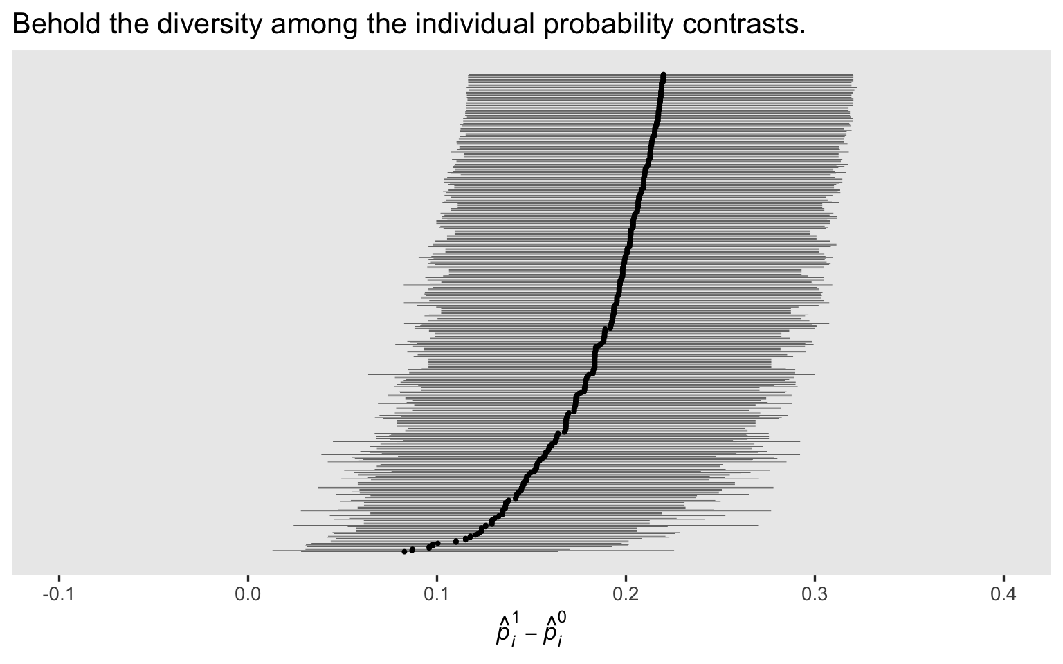
If you compare this plot with the original maximum-likelihood version from the last post, you’ll note our priors have reigned some of the posteriors in a bit, particularly the \(p_i^1 - p_i^0\) contrasts with the lowest rank. I don’t know that one solution is more correct than the other, but priors do change the model.

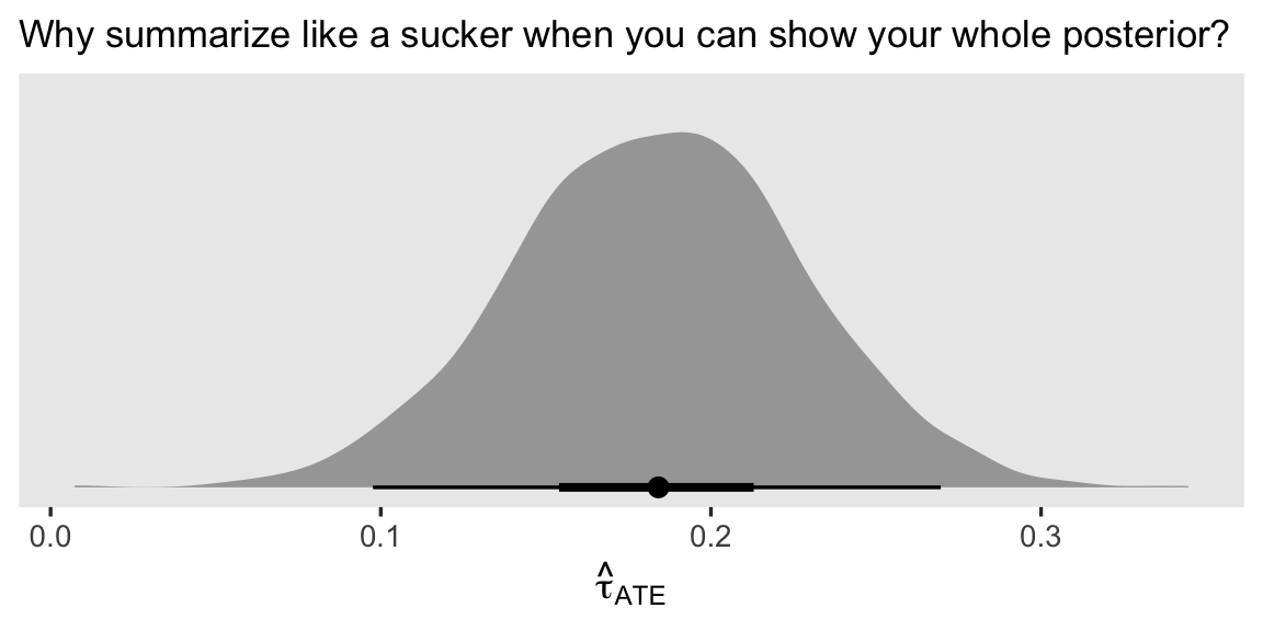
Since we’re plotting, we might also show the whole posterior distribution for the resulting \(\hat \tau_\text{ATE}\). Here we’ll base our wrangling workflow on the add_epred_draws() method, and then plot the results with help from the stat_halfeye() function.

nd %>% 
  add_epred_draws(fit4) %>% 
  ungroup() %>%
  select(tx, id, .draw, .epred) %>% 
  pivot_wider(names_from = tx, values_from = .epred) %>% 
  mutate(tau = `1` - `0`) %>% 
  group_by(.draw) %>% 
  summarise(ate = mean(tau)) %>% 
  
  ggplot(aes(x = ate)) +
  stat_halfeye(.width = c(.5, .95)) +
  scale_y_continuous(NULL, breaks = NULL) +
  labs(subtitle = "Why summarize like a sucker when you can show your whole posterior?",
       x = expression(hat(tau)[ATE]))

Recap

In this post, some of the main points we covered were:

• At a basic level, causal inference with Bayesian GLM’s isn’t that different from when we’re working as frequentists. The main difference is in the post-processing steps.
• We can compute identical results for the \(\tau_\text{ATE}\) or \(\tau_\text{CATE}\) with
  • a fitted()-based approach,
  • an as_draws_df()-based approach, or
  • a predictions()/avg_comparisons()-based approach.

In the next post, we’ll explore how our causal inference methods work with Poisson and negative-binomial models.

Thank a friend

Almost a year ago now, Mattan S. Ben-Shachar was the first person to show me how to compute the posterior for an ATE from a Bayesian logistic regression model (for the code, see here). Okay, technically his code used the Bernoulli likelihood, but whatever; they’re the same in this context. Anyway, I had never seen code like that before and, frankly, I found it baffling. That code example and the conceptual issues surrounding it are among the proximal causes of this entire blog series, and I’m very grateful.

Thank the reviewers

I’d like to publicly acknowledge and thank

• Isabella R. Ghement and
• Stephen J. Wild

for their kind efforts reviewing the draft of this post. Go team!

Do note the final editorial decisions were my own, and I do not think it would be reasonable to assume my reviewers have given blanket endorsements of the current version of this post.

Session information

sessionInfo()

## R version 4.3.0 (2023-04-21)
## Platform: aarch64-apple-darwin20 (64-bit)
## Running under: macOS Ventura 13.4
## 
## Matrix products: default
## BLAS:   /Library/Frameworks/R.framework/Versions/4.3-arm64/Resources/lib/libRblas.0.dylib 
## LAPACK: /Library/Frameworks/R.framework/Versions/4.3-arm64/Resources/lib/libRlapack.dylib;  LAPACK version 3.11.0
## 
## locale:
## [1] en_US.UTF-8/en_US.UTF-8/en_US.UTF-8/C/en_US.UTF-8/en_US.UTF-8
## 
## time zone: America/Chicago
## tzcode source: internal
## 
## attached base packages:
## [1] stats     graphics  grDevices utils     datasets  methods   base     
## 
## other attached packages:
##  [1] marginaleffects_0.12.0 tidybayes_3.0.4        brms_2.19.0            Rcpp_1.0.10            lubridate_1.9.2       
##  [6] forcats_1.0.0          stringr_1.5.0          dplyr_1.1.2            purrr_1.0.1            readr_2.1.4           
## [11] tidyr_1.3.0            tibble_3.2.1           ggplot2_3.4.2          tidyverse_2.0.0       
## 
## loaded via a namespace (and not attached):
##   [1] tensorA_0.36.2       rstudioapi_0.14      jsonlite_1.8.5       magrittr_2.0.3       TH.data_1.1-2       
##   [6] estimability_1.4.1   farver_2.1.1         nloptr_2.0.3         rmarkdown_2.22       vctrs_0.6.3         
##  [11] minqa_1.2.5          base64enc_0.1-3      blogdown_1.17        htmltools_0.5.5      distributional_0.3.2
##  [16] cellranger_1.1.0     sass_0.4.6           StanHeaders_2.26.27  bslib_0.5.0          htmlwidgets_1.6.2   
##  [21] plyr_1.8.8           sandwich_3.0-2       emmeans_1.8.6        zoo_1.8-12           cachem_1.0.8        
##  [26] igraph_1.4.3         mime_0.12            lifecycle_1.0.3      pkgconfig_2.0.3      colourpicker_1.2.0  
##  [31] Matrix_1.5-4         R6_2.5.1             fastmap_1.1.1        collapse_1.9.6       shiny_1.7.4         
##  [36] digest_0.6.31        numDeriv_2016.8-1.1  colorspace_2.1-0     ps_1.7.5             crosstalk_1.2.0     
##  [41] projpred_2.6.0       labeling_0.4.2       fansi_1.0.4          timechange_0.2.0     abind_1.4-5         
##  [46] mgcv_1.8-42          compiler_4.3.0       withr_2.5.0          backports_1.4.1      inline_0.3.19       
##  [51] shinystan_2.6.0      gamm4_0.2-6          highr_0.10           pkgbuild_1.4.1       MASS_7.3-58.4       
##  [56] gtools_3.9.4         loo_2.6.0            tools_4.3.0          httpuv_1.6.11        threejs_0.3.3       
##  [61] glue_1.6.2           callr_3.7.3          nlme_3.1-162         promises_1.2.0.1     grid_4.3.0          
##  [66] checkmate_2.2.0      reshape2_1.4.4       generics_0.1.3       gtable_0.3.3         tzdb_0.4.0          
##  [71] data.table_1.14.8    hms_1.1.3            utf8_1.2.3           pillar_1.9.0         ggdist_3.3.0        
##  [76] markdown_1.7         posterior_1.4.1      later_1.3.1          splines_4.3.0        lattice_0.21-8      
##  [81] survival_3.5-5       tidyselect_1.2.0     miniUI_0.1.1.1       knitr_1.43           arrayhelpers_1.1-0  
##  [86] gridExtra_2.3        bookdown_0.34        stats4_4.3.0         xfun_0.39            bridgesampling_1.1-2
##  [91] matrixStats_1.0.0    DT_0.28              rstan_2.21.8         stringi_1.7.12       yaml_2.3.7          
##  [96] boot_1.3-28.1        evaluate_0.21        codetools_0.2-19     cli_3.6.1            RcppParallel_5.1.7  
## [101] shinythemes_1.2.0    xtable_1.8-4         munsell_0.5.0        processx_3.8.1       jquerylib_0.1.4     
## [106] readxl_1.4.2         coda_0.19-4          svUnit_1.0.6         parallel_4.3.0       rstantools_2.3.1    
## [111] ellipsis_0.3.2       prettyunits_1.1.1    dygraphs_1.1.1.6     bayesplot_1.10.0     Brobdingnag_1.2-9   
## [116] lme4_1.1-33          mvtnorm_1.2-2        scales_1.2.1         xts_0.13.1           insight_0.19.2      
## [121] crayon_1.5.2         rlang_1.1.1          multcomp_1.4-24      shinyjs_2.1.0

References

Arel-Bundock, V. (2023). Bayesian analysis with brms. https://vincentarelbundock.github.io/marginaleffects/articles/brms.html
Bürkner, P.-C. (2017). brms: An R package for Bayesian multilevel models using Stan. Journal of Statistical Software, 80(1), 1–28. https://doi.org/10.18637/jss.v080.i01
Bürkner, P.-C. (2018). Advanced Bayesian multilevel modeling with the R package brms. The R Journal, 10(1), 395–411. https://doi.org/10.32614/RJ-2018-017
Bürkner, P.-C. (2022). brms: Bayesian regression models using ’Stan’. https://CRAN.R-project.org/package=brms
Bürkner, P.-C. (2023). brms reference manual, Version 2.19.0. https://CRAN.R-project.org/package=brms/brms.pdf
Bürkner, P.-C., Gabry, J., Kay, M., & Vehtari, A. (2022). posterior: Tools for working with posterior distributions. https://CRAN.R-project.org/package=posterior
Gelman, A., Hill, J., & Vehtari, A. (2020). Regression and other stories. Cambridge University Press. https://doi.org/10.1017/9781139161879
Horan, J. J., & Johnson, R. G. (1971). Coverant conditioning through a self-management application of the Premack principle: Its effect on weight reduction. Journal of Behavior Therapy and Experimental Psychiatry, 2(4), 243–249. https://doi.org/10.1016/0005-7916(71)90040-1
Kay, M. (2023). tidybayes: Tidy data and ’geoms’ for Bayesian models. https://CRAN.R-project.org/package=tidybayes
McElreath, R. (2020). Statistical rethinking: A Bayesian course with examples in R and Stan (Second Edition). CRC Press. https://xcelab.net/rm/statistical-rethinking/
Wilson, E., Free, C., Morris, T. P., Syred, J., Ahamed, I., Menon-Johansson, A. S., Palmer, M. J., Barnard, S., Rezel, E., & Baraitser, P. (2017). Internet-accessed sexually transmitted infection (e-STI) testing and results service: A randomised, single-blind, controlled trial. PLoS Medicine, 14(12), e1002479. https://doi.org/10.1371/journal.pmed.1002479
-
The exponential distribution is constrained to the positive real numbers, making it a good candidate prior distribution for
\(\sigma\)parameters. The gamma and lognormal distributions are just two of may other fine alternatives. For more discussion on the exponential prior, see McElreath ( 2020), chapter 4. ↩︎ -
The
\(\lambda\)parameter for the exponential distribution is often called the rate. There is an alternative parameterization which is expressed in terms of\(\beta\), often called the scale. These parameters are reciprocals of one another, meaning\(\beta = 1 / \lambda\), which also makes the scale the same as the mean. However, brms follows the base-R convention by using the\(\lambda\)parameterization. ↩︎ -
Why the confidence? Bear in mind I’m a psychology researcher. It’s my experience that continuous behavioral variables tend to have strong positive correlations over time. Granted, weight isn’t just a behavioral variable; it’s physiological too. Even still, I’m a human who has weighed himself many times over the years, and I’ve observed the gross trends in other peoples proportions. Even within the context of a weight-loss intervention, weight at baseline is going to have a strong positive correlation with post-intervention weight. ↩︎
Unlike with the frequentist base-R
glm()function,brms::brm()also supports Bernoulli regression for binary data. Just setfamily = bernoulli. Personally, I prefer the binomial likelihood because of how it seamlessly generalizes to aggregated binomial counts. The curious reader might try it both ways. ↩︎
- Posted on:
- April 30, 2023
- Length:
- 40 minute read, 8436 words