Causal inference with count regression

In the third post in this series, we extended out counterfactual causal-inference framework to binary outcome data. We saw how logistic regression complicated the approach, particularly when using baseline covariates. In this post, we’ll practice causal inference with unbounded count data, using the Poisson and negative-binomial likelihoods.

We need data

We’ll be working with a subset of the epilepsy data from the brms package. Based on the brms documentation (execute ?epilepsy), the data have their proximal origins in a ( 1990) Biometrics paper by Thall and Vail. However, Thall and Vail cited an earlier paper by Leppik et al. ( 1985) as the ultimate origin.¹ Here we load our primary packages, adjust the global plotting theme, load the epilepsy data, and take a peek.

# packages
library(tidyverse)
library(brms)
library(flextable)
library(GGally)
library(broom)
library(ggdist)
library(lmtest)
library(sandwich)
library(tidybayes)
library(marginaleffects)
library(patchwork)

# adjust the global theme
theme_set(theme_gray(base_size = 12) +
            theme(panel.grid = element_blank()))

# load the data
data(package = "brms", epilepsy)

# what?
glimpse(epilepsy)

## Rows: 236
## Columns: 9
## $ Age     <dbl> 31, 30, 25, 36, 22, 29, 31, 42, 37, 28, 36, 24, 23, 36, 26, 26, 28, 31, 32, 21, 29, 21, 32, …
## $ Base    <dbl> 11, 11, 6, 8, 66, 27, 12, 52, 23, 10, 52, 33, 18, 42, 87, 50, 18, 111, 18, 20, 12, 9, 17, 28…
## $ Trt     <fct> 0, 0, 0, 0, 0, 0, 0, 0, 0, 0, 0, 0, 0, 0, 0, 0, 0, 0, 0, 0, 0, 0, 0, 0, 0, 0, 0, 0, 1, 1, 1,…
## $ patient <fct> 1, 2, 3, 4, 5, 6, 7, 8, 9, 10, 11, 12, 13, 14, 15, 16, 17, 18, 19, 20, 21, 22, 23, 24, 25, 2…
## $ visit   <fct> 1, 1, 1, 1, 1, 1, 1, 1, 1, 1, 1, 1, 1, 1, 1, 1, 1, 1, 1, 1, 1, 1, 1, 1, 1, 1, 1, 1, 1, 1, 1,…
## $ count   <dbl> 5, 3, 2, 4, 7, 5, 6, 40, 5, 14, 26, 12, 4, 7, 16, 11, 0, 37, 3, 3, 3, 3, 2, 8, 18, 2, 3, 13,…
## $ obs     <fct> 1, 2, 3, 4, 5, 6, 7, 8, 9, 10, 11, 12, 13, 14, 15, 16, 17, 18, 19, 20, 21, 22, 23, 24, 25, 2…
## $ zAge    <dbl> 0.42499501, 0.26528351, -0.53327400, 1.22355252, -1.01240850, 0.10557201, 0.42499501, 2.1818…
## $ zBase   <dbl> -0.757172825, -0.757172825, -0.944403322, -0.869511123, 1.302362646, -0.158035233, -0.719726…

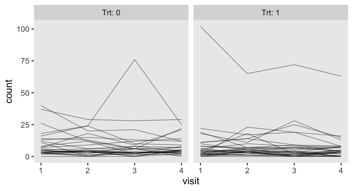
The original study was designed to see how well the anti-convulsant drug progabide reduced epileptic seizures in persons who experienced simple or complex partial seizures. After a baseline assessment, participants were randomized into treatment groups in which they received either progabide (Trt == 1) or a placebo (Trt == 0). The primary outcome variable in the data is count, which is the number of epileptic seizures each participant had had since their last visit. Following their baseline assessments, participants came back every two weeks for assessments, which are denoted by the factor variable visit. To get a sense of the data, here are the seizures counts over the four assessment points, by treatment group.

epilepsy %>% 
  mutate(visit = as.double(visit)) %>% 
  
  ggplot(aes(x = visit, y = count, group = patient)) +
  geom_line(linewidth = 1/3, alpha = 1/2) +
  facet_wrap(~ Trt, labeller = label_both)

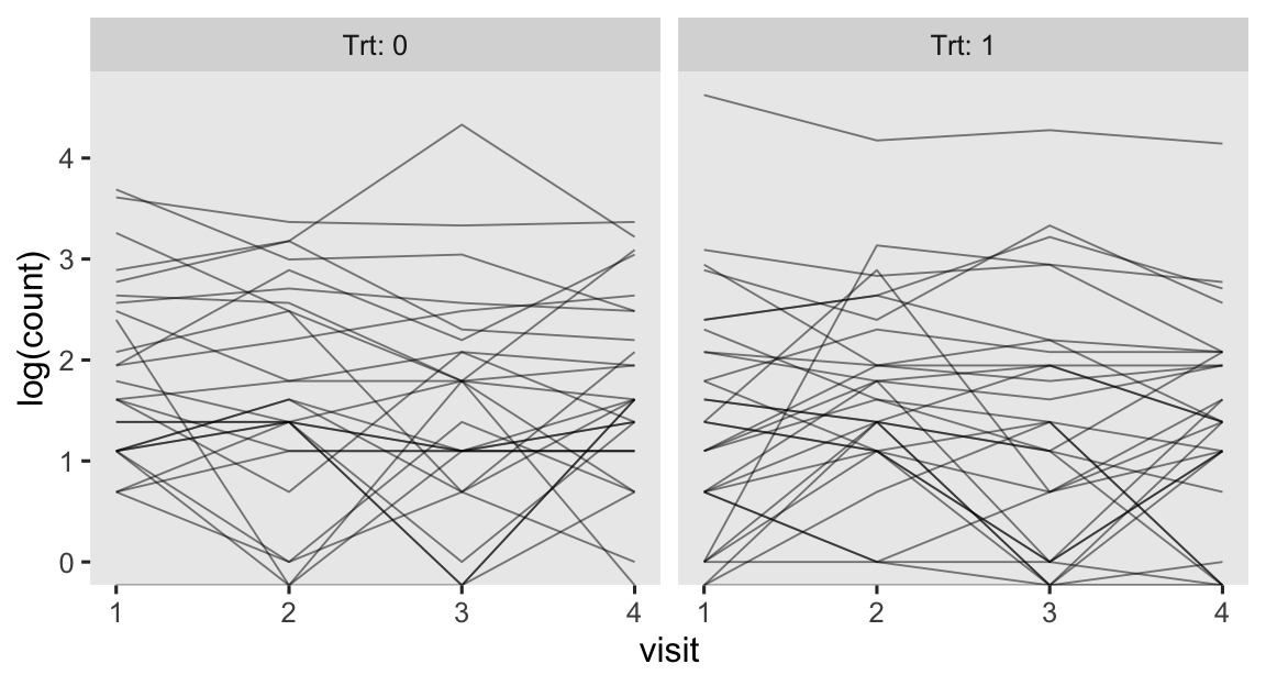
As we’ll see later, researchers often model counts like this with the log link. So here’s the same data, but with count on the log scale.

epilepsy %>% 
  mutate(visit = as.double(visit)) %>% 
  
  ggplot(aes(x = visit, y = log(count), group = patient)) +
  geom_line(linewidth = 1/3, alpha = 1/2) +
  facet_wrap(~ Trt, labeller = label_both)

Here are some of the sample statistics, by Trt and visit, in a Table 1 type format.

epilepsy %>% 
  group_by(Trt, visit) %>% 
  summarise(mean = mean(count),
            variance = var(count),
            min = min(count),
            max = max(count)) %>% 
  mutate_if(is.double, round, digits = 1) %>%
  as_grouped_data(groups = c("Trt")) %>%
  flextable()

It’ll become apparent why we computed variances instead of standard deviations in a little bit.

Subset, wrangle, inspect.

It’d be cool to play around modeling the data from all four time points,² but that would be too much of a distraction from our central goal. So we’re going to subset the data to only include the rows for the fourth assessment period (i.e., visit == 4). We’ll call the reduced data set ep4.

ep4 <- epilepsy %>% 
  # subset
  filter(visit == 4) %>% 
  # add two transformed variables
  mutate(lcBase = log(Base) - mean(log(Base)),
         lcAge = log(Age) - mean(log(Age)))

# what?
glimpse(ep4)

## Rows: 59
## Columns: 11
## $ Age     <dbl> 31, 30, 25, 36, 22, 29, 31, 42, 37, 28, 36, 24, 23, 36, 26, 26, 28, 31, 32, 21, 29, 21, 32, …
## $ Base    <dbl> 11, 11, 6, 8, 66, 27, 12, 52, 23, 10, 52, 33, 18, 42, 87, 50, 18, 111, 18, 20, 12, 9, 17, 28…
## $ Trt     <fct> 0, 0, 0, 0, 0, 0, 0, 0, 0, 0, 0, 0, 0, 0, 0, 0, 0, 0, 0, 0, 0, 0, 0, 0, 0, 0, 0, 0, 1, 1, 1,…
## $ patient <fct> 1, 2, 3, 4, 5, 6, 7, 8, 9, 10, 11, 12, 13, 14, 15, 16, 17, 18, 19, 20, 21, 22, 23, 24, 25, 2…
## $ visit   <fct> 4, 4, 4, 4, 4, 4, 4, 4, 4, 4, 4, 4, 4, 4, 4, 4, 4, 4, 4, 4, 4, 4, 4, 4, 4, 4, 4, 4, 4, 4, 4,…
## $ count   <dbl> 3, 3, 5, 4, 21, 7, 2, 12, 5, 0, 22, 4, 2, 14, 9, 5, 3, 29, 5, 7, 4, 4, 5, 8, 25, 1, 2, 12, 8…
## $ obs     <fct> 178, 179, 180, 181, 182, 183, 184, 185, 186, 187, 188, 189, 190, 191, 192, 193, 194, 195, 19…
## $ zAge    <dbl> 0.42499501, 0.26528351, -0.53327400, 1.22355252, -1.01240850, 0.10557201, 0.42499501, 2.1818…
## $ zBase   <dbl> -0.757172825, -0.757172825, -0.944403322, -0.869511123, 1.302362646, -0.158035233, -0.719726…
## $ lcBase  <dbl> -0.75635379, -0.75635379, -1.36248959, -1.07480752, 1.03540568, 0.14158780, -0.66934241, 0.7…
## $ lcAge   <dbl> 0.11420370, 0.08141387, -0.10090768, 0.26373543, -0.22874106, 0.04751232, 0.11420370, 0.4178…

The glimpse() output helps clarify there were 59 unique participants in this study. If you use the count() function, you’ll find \(n = 28\) are in the placebo condition, and the remaining \(n = 31\) got the active treatment. The data also contain information from the baseline assessment in the Base column, which has the epileptic seizure counts during the 8-week period before the baseline assessment. Bear in mind the counts in the count column were for a 2-week period, which means we’d expect the values in Base to be at least 4 times larger than those in count. But since they’re all seizure counts, it seems like we’d still expect the two variables to have a strong positive correlation. The other baseline covariate in the data, which was also considered by Thall & Vail ( 1990), is age measured in years (Age). The data from the brms package includes standardized version of these variables in the zBase and zAge columns. Thall and Vail, however, used log-transformed versions of these variables, which is what we’ll do in this blog post. Thus, our new variable lcBase is the log-transformed and mean-centered version of Base, and lcAge is the log-transformed and mean-centered version of Age.

Since it can be difficult to think in terms of the mean values of log-transformed variables, here are what the means of those log-transformed values are, when exponentiated back into their original metric.³

ep4 %>% 
  summarise(`exponentiated_mean_of_log(Base)` = mean(log(Base)) %>% exp(),
            `exponentiated_mean_of_log(Age)` = mean(log(Age)) %>% exp()) 

##   exponentiated_mean_of_log(Base) exponentiated_mean_of_log(Age)
## 1                        23.43543                       27.65436

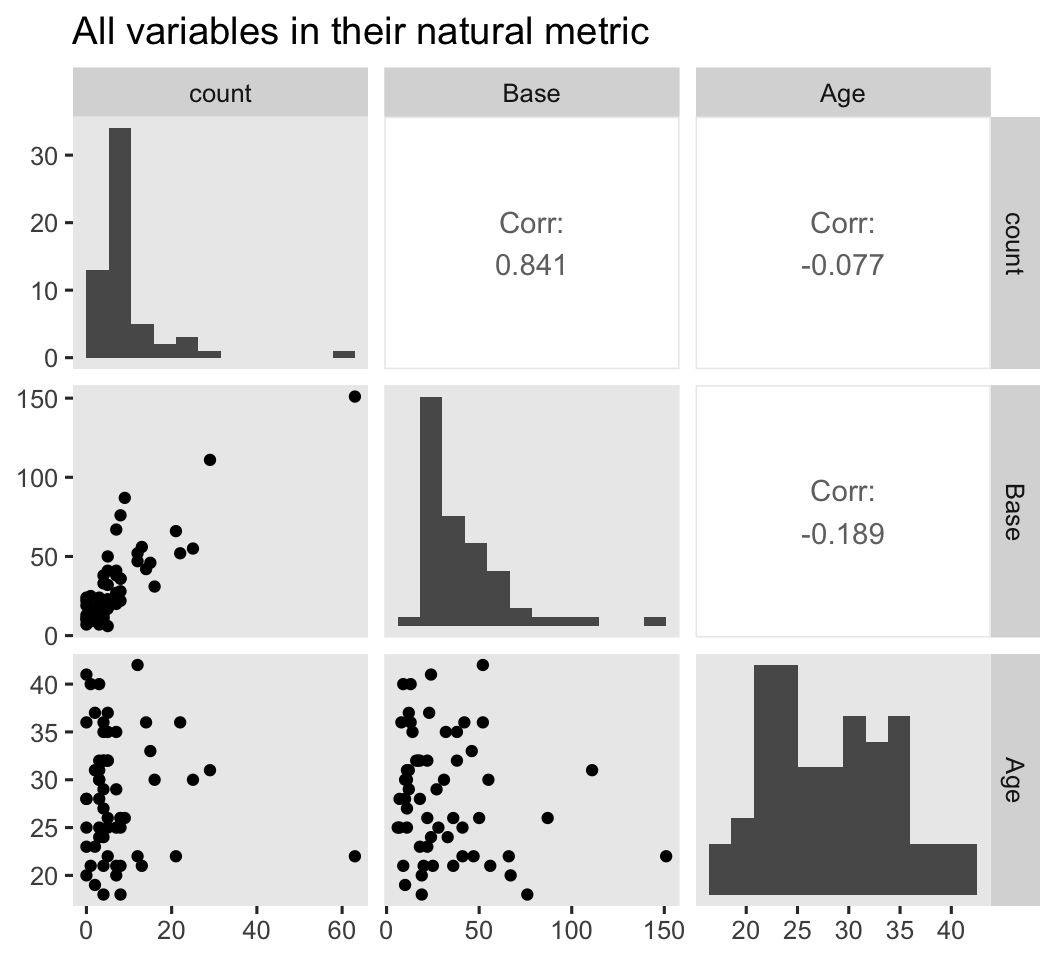
We might want to get a further sense of the outcome variable and the two baseline covariates with a couple pairs plot with help from the GGally package ( Schloerke et al., 2021). We’ll look at them in both their natural metrics, and on the log scale.

# natural metric
ep4 %>% 
  select(count, Base, Age) %>% 
  ggpairs(diag = list(continuous = wrap("barDiag", bins = 12)),
          upper = list(continuous = wrap("cor", stars = FALSE))) +
  ggtitle("All variables in their natural metric")

# log scale
ep4 %>% 
  mutate(lcount = log(count)) %>% 
  select(lcount, lcBase, lcAge) %>% 
  ggpairs(diag = list(continuous = wrap("barDiag", bins = 12)),
          upper = list(continuous = wrap("cor", stars = FALSE))) +
  ggtitle("All variables on the log scale")

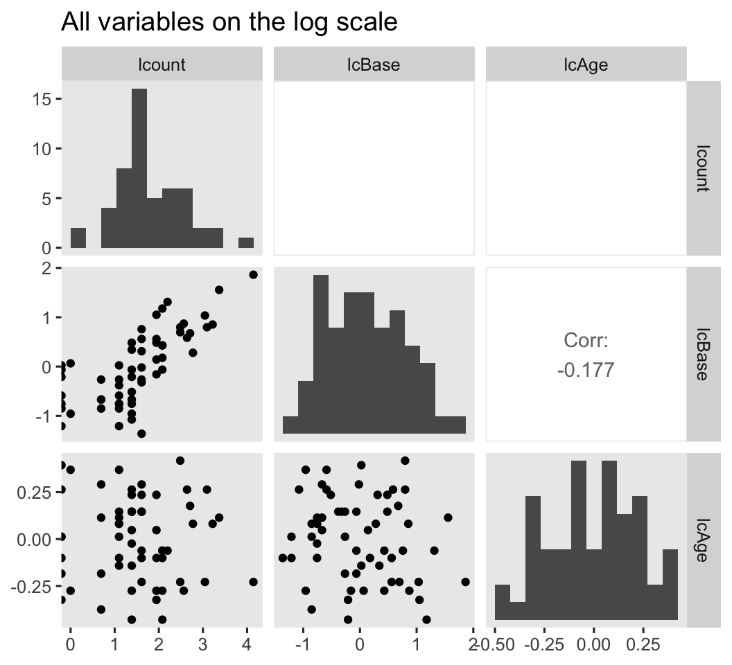
Because several of the count values were zero, transforming them to the log scale resulted in \(-\infty\) values. ggpairs() dropped those values from the scatter plots and histograms, but otherwise returned the plots for the other values. However, those \(-\infty\) values kept us from computing the Pearson’s correlations between log(count) and the other two variables. If you’re willing to settle for listwise removal of those values, here are the Pearson’s correlation estimates for the remaining cases.

ep4 %>% 
  mutate(lcount = log(count)) %>% 
  filter(lcount != -Inf) %>% 
  summarise(`r[lcBase, lcount]` = cor(lcBase, lcount),
            `r[lcAge, lcount]` = cor(lcAge, lcount))

##   r[lcBase, lcount] r[lcAge, lcount]
## 1         0.7594784      -0.06570049

Model framework

Our well-named focal variable count is an unbounded count. Technically all count variables are bounded in that their lower limit is always zero.⁴ By unbounded count, I mean there is no clearly-defined upper limit such as with binomial data. When you have unbounded counts, the two most popular likelihoods are the Poisson and the negative-binomial. The Poisson likelihood is parsimonious in that it contains a single parameter \(\lambda\), which is both the mean and the variance. As such, the Poisson likelihood assumes the variance scales perfectly with the mean, which is often called the equidispersion assumption. If you look back above at the sample statistics, you’ll notice the variances for count were a lot larger than the means at all time points and for both conditions, which doesn’t bode well for that equidispersion assumption.⁵ Happily, the negative-binomial likelihood provides an alternative where its second parameter \(\phi\) accounts for additional variance above what we’d expect from the Poisson. For the sake of practice, in this blog post we’ll analyze these data from both frequentist and Bayesian perspectives, and also with the Poisson and negative-binomial likelihoods. To complicate matters even further, we’ll also analyze the data with ANOVA- and ANCOVA-type frameworks. Putting all three binaries together, we’ll end up fitting and post-processing 6 models in total:

tibble(
  name = c(str_c("fit", 1:4), str_c("brm", 1:2)),
  framework = rep(c("frequentist", "Bayesian"), times = c(4, 2)),
  model = rep(c("ANOVA", "ANCOVA", "ANOVA", "ANCOVA"), times = c(2, 2, 1, 1)),
  likelihood = c("Poisson", "negative-binomial", "Poisson", "negative-binomial", "negative-binomial", "Poisson")
) %>%
  flextable() %>%
  autofit()

For the sake of space, well only fit two Bayesian models. My hope is by the time we’re in that section, you’ll get the gist of what’s going on. For the frequentist models, we’ll also discuss the issue of robust standard errors, which won’t apply to our Bayesian models.

We start as frequentists.

Frequentist models.

Define the equations and fit.

Our Poisson ANOVA model will be of the form

$$ \begin{align*} \text{count}_i & \sim \operatorname{Poisson}(\lambda_i) \\ \log(\lambda_i) & = \beta_0 + \beta_1 \text{Trt}_i, \end{align*} $$

where we use the conventional log link to ensure we only make positive predictions. The \(\beta_0\) parameter is the placebo mean on the log scale, and \(\beta_1\) is the deviation from that mean on log-scale units for those in the active treatment group. In a similar way, the negative-binomial version of our ANOVA model will be of the form

$$ \begin{align*} \text{count}_i & \sim \operatorname{Negative Binomial}(\mu_i, \phi) \\ \log(\mu_i) & = \beta_0 + \beta_1 \text{Trt}_i, \end{align*} $$

where instead of \(\lambda_i\), we now use the notation of \(\mu_i\). We continue to follow convention with the log link, and the \(\beta_0\) and \(\beta_0\) parameters have largely the same interpretation as before.

Our frequentist Poisson ANCOVA model will be of the form

$$ \begin{align*} \text{count}_i & \sim \operatorname{Poisson}(\lambda_i) \\ \log(\lambda_i) & = \beta_0 + \beta_1 \text{Trt}_i + \beta_2 \text{lcBase}_i + \beta_3 \text{lcAge}_i, \end{align*} $$

where we use the log-transformed and mean-centered versions of baseline seizure counts (lcBase) and age (lcAge). In a similar way, the negative-binomial version of the ANCOVA model will be

$$ \begin{align*} \text{count}_i & \sim \operatorname{Negative Binomial}(\mu_i, \phi) \\ \log(\mu_i) & = \beta_0 + \beta_1 \text{Trt}_i + \beta_2 \text{lcBase}_i + \beta_3 \text{lcAge}_i. \end{align*} $$

We can fit the frequentist Poisson models with the good-old base R glm() function, provided we set family = poisson. The frequentist negative-binomial models require the glm.nb() function from the MASS package ( Ripley, 2022; Venables & Ripley, 2002). You’ll note that instead of opening MASS directly with library(), we’re instead using the focused MASS::glm.nb() syntax. This is because MASS can create conflicts with some of the tidyverse functions, and I’d like to avoid those complications.

# Poisson ANOVA
fit1 <- glm(
  data = ep4,
  family = poisson,
  count ~ Trt)

# NB ANOVA
fit2 <- MASS::glm.nb(
  data = ep4,
  count ~ Trt)

# Poisson ANCOVA
fit3 <- glm(
  data = ep4,
  family = poisson,
  count ~ Trt + lcBase + lcAge)

# NB ANCOVA
fit4 <- MASS::glm.nb(
  data = ep4,
  count ~ Trt + lcBase + lcAge)

For the sake of space, I’m not going to show all the summary() output for these models. Here’s a table of their \(\beta\) coefficient summaries, instead.

bind_rows(tidy(fit1), tidy(fit2), tidy(fit3), tidy(fit4)) %>% 
  mutate(fit = rep(str_c("fit", 1:4), times = c(2, 2, 4, 4))) %>% 
  select(fit, everything()) %>% 
  mutate_if(is.double, round, digits = 3) %>%
  as_grouped_data(groups = c("fit")) %>%
  flextable()

We should note that the standard errors in that table are all based on conventional maximum likelihood (ML) estimation, which are typically fine defaults, to my eye. However, that equidispersion assumption for the Poisson models can result in very small standard errors, relative to those from their negative-binomial alternatives. Sometimes researchers prefer using so-called robust standard errors, instead. We can compute those with help from the coeftest() function from the lmtest package ( Hothorn et al., 2022; Zeileis & Hothorn, 2002). By setting vcov = vcovHC, we are requesting the so-called HC3 sandwich standard errors, via the sandwich package ( Zeileis, 2004, 2006; Zeileis et al., 2020; Zeileis & Lumley, 2022). Here’s how all this works for our Poisson ANOVA model fit1, within the context of the tidy() function.

coeftest(fit1, vcov = vcovHC) %>% 
  tidy()

## # A tibble: 2 × 5
##   term        estimate std.error statistic  p.value
##   <chr>          <dbl>     <dbl>     <dbl>    <dbl>
## 1 (Intercept)    2.07      0.184    11.3   2.13e-29
## 2 Trt1          -0.171     0.358    -0.479 6.32e- 1

If you compare those standard errors to the values in the first two rows of the table, above, you’ll see they’re about 3 times larger. Larger standard errors will result in wider (i.e., less certain) 95% confidence intervals. Now we have a sense of how this works, let’s compare the effects of the standard errors on the 95% confidence intervals in a coefficient plot.

bind_rows(
  # conventional ML SE's
  tibble(name = str_c("fit", 1:4),
         model = rep(c("ANOVA", "ANCOVA"), each = 2), 
         likelihood = rep(c("Poisson", "NB"), times = 2),
         se = "ML") %>% 
    mutate(fit = map(name, get)) %>% 
    mutate(tidy = map(fit, tidy, conf.int = TRUE)),
  # sandwich SE's
  tibble(name = str_c("fit", 1:4),
         model = rep(c("ANOVA", "ANCOVA"), each = 2), 
         likelihood = rep(c("Poisson", "NB"), times = 2),
         se = "sandwich") %>% 
    mutate(fit = map(name, get)) %>% 
    mutate(tidy = map(fit, ~tidy(coeftest(., vcov = vcovHC), conf.int = TRUE)))
) %>% 
  select(-fit) %>% 
  unnest(tidy) %>% 
  mutate(model      = factor(model, levels = c("ANOVA", "ANCOVA")),
         likelihood = factor(likelihood, levels = c("Poisson", "NB")),
         beta       = case_when(
    term == "(Intercept)" ~ "beta[0]",
    term == "Trt1"        ~ "beta[1]",
    term == "lcBase"      ~ "beta[2]",
    term == "lcAge"       ~ "beta[3]"
  )) %>% 
  
  ggplot(aes(x = estimate, xmin = conf.low, xmax = conf.high, y = model, color = se)) +
  geom_pointinterval(position = position_dodge(width = -0.4)) +
  scale_color_viridis_d(expression(italic(SE)*"'s:"), option = "A", end = .5) +
  scale_x_continuous(expand = expansion(mult = 0.25)) +
  labs(x = "parameter space",
       y = NULL) +
  facet_grid(likelihood ~ beta, labeller = label_parsed, scales = "free_x") +
  theme(axis.text.y = element_text(hjust = 0),
        legend.position = "top")

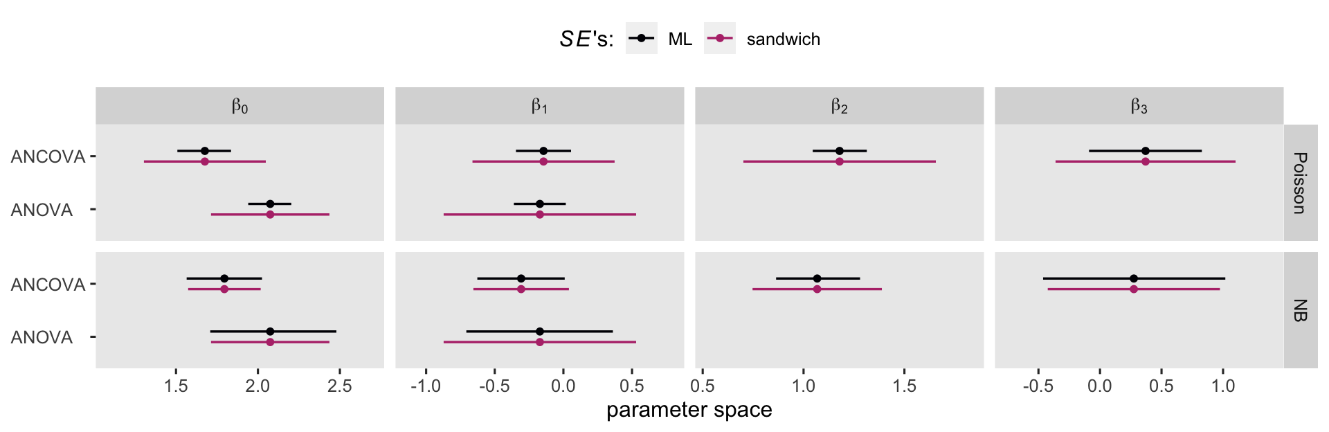
Overall, the sandwich standard errors resulted in narrower CI’s in the Poisson models, particularly for the Poisson ANOVA. But the sandwich standard errors did change the results for the negative-binomial models, too. As we will see in the next few sections, the choice of one’s likelihood and standard error method will influence causal inference. Sadly, I can’t tell you what the right choice is for your research program. All I can do, here, is let you know about some of your options.

Can the \(\beta\) coefficients help us estimate the ATE?

Much like with logistic regression models, the \(\beta_1\) parameter alone cannot give us the average treatment effect (ATE) for either the Poisson or negative-binomial likelihoods. However, we can use a combination of the \(\beta_0\) and \(\beta_1\) parameters to give us the ATE, when they are from the ANOVA models. The formula is

$$\exp(\beta_0 + \beta_1) - \exp(\beta_0).$$

The reason we exponentiate is to convert the predictions from the log-scale back onto the natural count scale. Here’s how to execute that formula in code, with our Poisson and negative-binomial ANOVA-type models.

exp(coef(fit1)[1] + coef(fit1)[2]) - exp(coef(fit1)[1])  # Poisson ANOVA 

## (Intercept) 
##   -1.254608

exp(coef(fit2)[1] + coef(fit2)[2]) - exp(coef(fit2)[1])  # negative-binomial ANOVA 

## (Intercept) 
##   -1.254608

Sadly, the Poisson and negative-binomial ANOCVA-type models give us no such way to compute the ATE. We can, however, compute some form of the conditional average treatment effect (CATE). For example, given how both of the covariates in our ANCOVA models are mean centered, we can simply use the equation from above,

$$\exp(\beta_0 + \beta_1) - \exp(\beta_0),$$

to compute the Poisson and negative-binomial CATE for a person of average baseline seizure counts (about 23.4) and age (about 27.7).

exp(coef(fit3)[1] + coef(fit3)[2]) - exp(coef(fit3)[1])  # Poisson ANCOVA 

## (Intercept) 
##  -0.7203651

exp(coef(fit4)[1] + coef(fit4)[2]) - exp(coef(fit4)[1])  # negative-binomial ANCOVA 

## (Intercept) 
##   -1.595425

Note how the ANCOVA models give different results from one another, and different results from their ANOVA counterparts. As we’ve seen in other contexts,

$$\tau_\text{ATE} \neq \tau_\text{CATE},$$

for Poisson and negative-binomial models using the conventional log link.

Compute \(\mathbb E (\lambda_i^1 - \lambda_i^0)\) or \(\mathbb E (\mu_i^1 - \mu_i^0)\).

When we have unbounded count data, it’s still the case that

$$\tau_\text{ATE} = \mathbb E (y_i^1 - y_i^0).$$

Somewhat similar to what we saw with logistic regression models, we have some technical quirks to consider. Unbounded count data can take on positive integer values, sometimes denoted \(\mathbb N_0\) (natural numbers starting from zero). Therefore their contrasts, such as \(y_i^1 - y_i^0\), can in principle take on any integer value, positive or negative, sometimes denoted \(\mathbb Z\). When you take the mean for several positive integer values, you get a positive real number, sometimes denoted \(\mathbb R^+\). But when you either take the mean of the mean of several positive-integer contrasts, or make a contrast of two integer averages, you can in principle get any real number, sometimes denoted \(\mathbb R\).

Our Poisson framework returns linear models for \(\log(\lambda_i)\), and our negative-binomial framework returns linear models for \(\log(\mu_i)\). After exponentiation, both \(\lambda_i\) and \(\mu_i\) can take on positive real numbers \((\mathbb R^+)\), and their contrasts can take on positive or negative real numbers \((\mathbb R)\). For example, see what happens when we use predict() for the Poisson ANOVA, fit1.

nd <- ep4 %>% 
  select(patient) %>% 
  expand_grid(Trt = factor(0:1))

# compute
predict(fit1, 
        newdata = nd,
        se.fit = TRUE,
        # request the lambda metric;
        # the default is on the log scale
        type = "response") %>% 
  data.frame() %>% 
  bind_cols(nd) %>% 
  # look at the first 6 rows
  head()

##        fit    se.fit residual.scale patient Trt
## 1 7.964286 0.5333280              1       1   0
## 2 6.709677 0.4652324              1       1   1
## 3 7.964286 0.5333280              1       2   0
## 4 6.709677 0.4652324              1       2   1
## 5 7.964286 0.5333280              1       3   0
## 6 6.709677 0.4652324              1       3   1

The fit column contains the \(\hat \lambda_i\) values, rather than \(\hat y_i\) values we like to think of when making causal inferences. This won’t be a problem, though. It turns out that when you take the average of the contrast of these values, you still get an estimate of the ATE (see Section 18.4 of Greene, 2018). Thus within the context of our Poisson ANOVA model,

$$\tau_\text{ATE} = \mathbb E (y_i^1 - y_i^0) = {\color{blueviolet}{\mathbb E (\lambda_i^1 - \lambda_i^0)}}.$$

In a similar way for our negative-binomial ANOVA model,

$$\tau_\text{ATE} = \mathbb E (y_i^1 - y_i^0) = {\color{blueviolet}{\mathbb E (\mu_i^1 - \mu_i^0)}}.$$

The same principles will hold for our Poisson and negative-binomial ANCOVA models. To expand this framework to ANCOVA-type models, let \(\mathbf C_i\) stand a vector of continuous covariates and let \(\mathbf D_i\) stand a vector of discrete covariates, both of which vary across the \(i\) cases. We can use these to help estimate the ATE from the Poisson ANCOVA with the formula

$$\tau_\text{ATE} = \mathbb E (y_i^1 - y_i^0 \mid \mathbf C_i, \mathbf D_i) = {\color{blueviolet}{\mathbb E (\lambda_i^1 - \lambda_i^0 \mid \mathbf C_i, \mathbf D_i)}},$$

where \(\lambda_i^1\) and \(\lambda_i^0\) are the counterfactual rates for each of the \(i\) cases, estimated in light of their covariate values. In the same way, we estimate the ATE from the negative-binomial ANCOVA with the formula

$$\tau_\text{ATE} = \mathbb E (y_i^1 - y_i^0 \mid \mathbf C_i, \mathbf D_i) = {\color{blueviolet}{\mathbb E (\mu_i^1 - \mu_i^0 \mid \mathbf C_i, \mathbf D_i)}}.$$

This, again, is sometimes called standardization or g-computation, this time applied to count models.

Before we practice computing our \(\hat \tau_\text{ATE}\) values, we should spend some time with the counterfactual \(\hat \lambda_i^1\), \(\hat \lambda_i^0\), \(\hat \mu_i^1\), and \(\hat \mu_i^0\) values. As we’ve done in previous posts, we can compute those with the marginaleffects::predictions() function. We’ll start with the counterfactual predictions from the Poisson models.

models <- c("ANOVA", "ANCOVA")
ses <- c("ML", "sandwich")

# update the predictor grid to include the covariates
nd <- ep4 %>% 
  select(patient, lcBase, lcAge) %>% 
  expand_grid(Trt = factor(0:1))

# compute and wrangle
bind_rows(
  predictions(fit1, newdata = nd),
  predictions(fit1, newdata = nd, vcov = "HC3"),
  predictions(fit3, newdata = nd),
  predictions(fit3, newdata = nd, vcov = "HC3")
) %>% 
  data.frame() %>% 
  mutate(y     = ifelse(Trt == 0, "hat(lambda)^0", "hat(lambda)^1"),
         model = rep(models, each = 2) %>% rep(., each = n() / 4) %>% factor(., levels = models),
         se    = rep(ses, times = 2) %>% rep(., each = n() / 4) %>% factor(., levels = ses)) %>% 
  
  # plot!
  ggplot(aes(x = estimate, y = reorder(patient, estimate))) +
  geom_interval(aes(xmin = conf.low, xmax = conf.high, color = y),
                position = position_dodge(width = -0.2),
                size = 1/5) +
  geom_point(aes(color = y, shape = y),
             size = 2) +
  scale_color_viridis_d(NULL, option = "A", begin = .3, end = .6,
                        labels = scales::parse_format()) +
  scale_shape_manual(NULL, values = c(20, 18),
                     labels = scales::parse_format()) +
  scale_y_discrete(breaks = NULL) +
  labs(subtitle = "Counterfactual Poisson rates, by model type and standard error method",
       x = expression(lambda[italic(i)]),
       y = "patient (ranked)") +
  coord_cartesian(xlim = c(0, 50)) +
  theme(legend.background = element_blank(),
        legend.position = c(.9, .85)) +
  facet_grid(se ~ model)

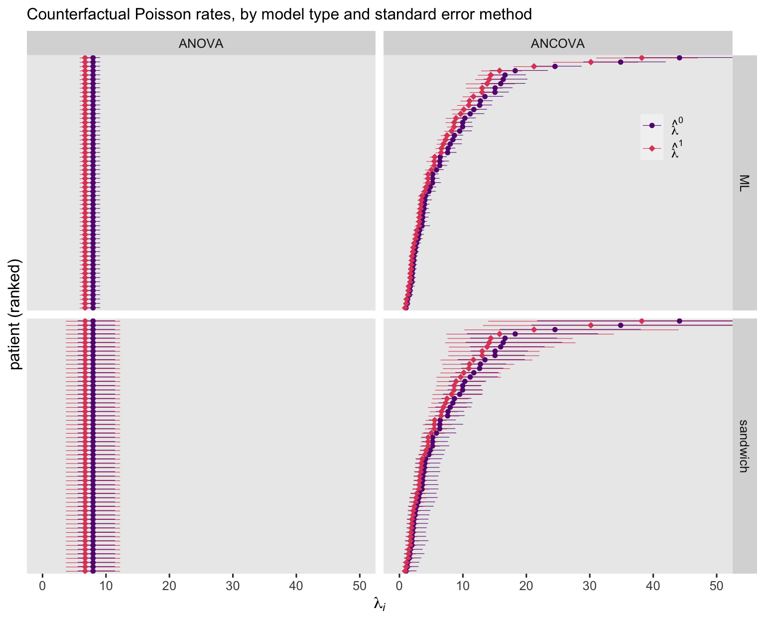
Unsurprisingly, the ANOVA-based point estimates are the same for all participants. Yet the estimates for the ANCOVA model showed great diversity among the participants. As to the 95% CI’s, they were markedly wider when based on the sandwich standard errors, suggesting the Poisson models did not adequately account for the overdispersion in the data. Now look at the negative-binomial versions of the figure.

# compute and wrangle
bind_rows(
  predictions(fit2, newdata = nd),
  predictions(fit2, newdata = nd, vcov = "HC3"),
  predictions(fit4, newdata = nd),
  predictions(fit4, newdata = nd, vcov = "HC3")
) %>% 
  data.frame() %>% 
  mutate(y     = ifelse(Trt == 0, "hat(mu)^0", "hat(mu)^1"),
         model = rep(models, each = 2) %>% rep(., each = n() / 4) %>% factor(., levels = models),
         se    = rep(ses, times = 2) %>% rep(., each = n() / 4) %>% factor(., levels = ses)) %>% 
  
  # plot!
  ggplot(aes(x = estimate, y = reorder(patient, estimate))) +
  geom_interval(aes(xmin = conf.low, xmax = conf.high, color = y),
                position = position_dodge(width = -0.2),
                size = 1/5) +
  geom_point(aes(color = y, shape = y),
             size = 2) +
  scale_color_viridis_d(NULL, option = "A", begin = .3, end = .6,
                        labels = scales::parse_format()) +
  scale_shape_manual(NULL, values = c(20, 18),
                     labels = scales::parse_format()) +
  scale_y_discrete(breaks = NULL) +
  labs(subtitle = "Counterfactual negative-binomial means, by model type and standard error method",
       x = expression(mu[italic(i)]),
       y = "patient (ranked)") +
  coord_cartesian(xlim = c(0, 50)) +
  theme(legend.background = element_blank(),
        legend.position = c(.9, .85)) +
  facet_grid(se ~ model)

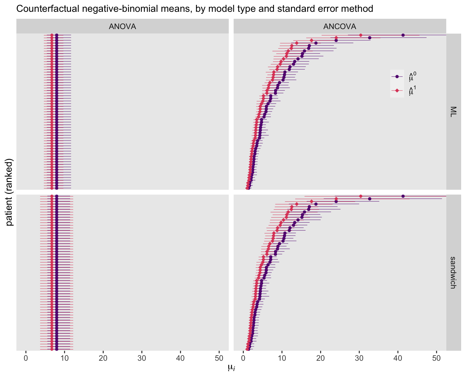
For the ANOVA models, the negative-binomial point estimates are identical to those from the Poisson variants. For the ANCOVA models, the negative-binomial point estimates are similar to their Poisson counterparts, but not quite identical. Overall, the negative-binomial 95% CI’s are wider than those from the Poisson models, but much less notably so when computed with the sandwich standard errors.

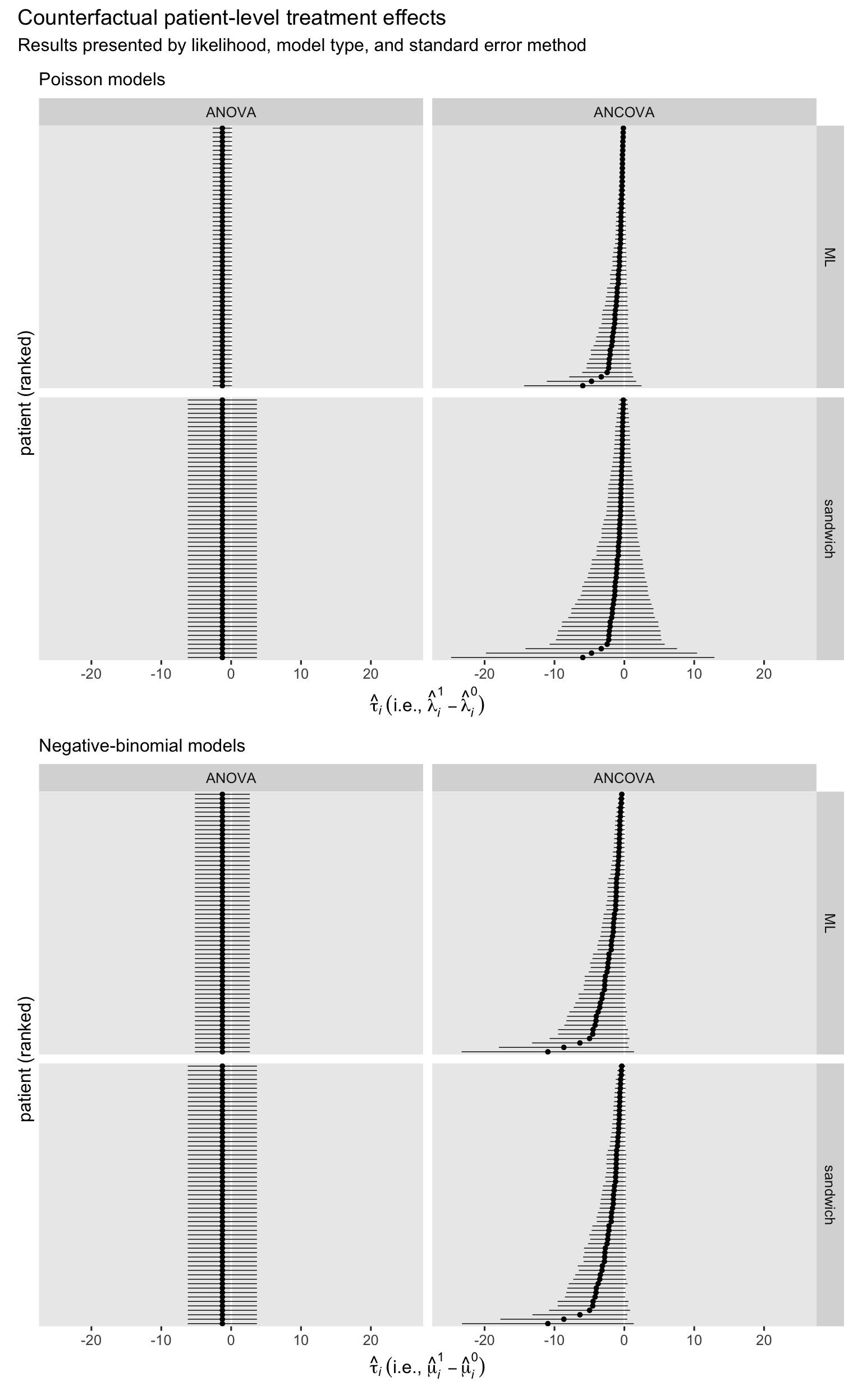
Now we use the marginaleffects::comparisons() function to compute the patient-level treatment effect estimates for each combination of likelihood, model type, and standard error method.

# Poisson
p1 <- bind_rows(
  comparisons(fit1, variables = "Trt", by = "patient"),
  comparisons(fit1, variables = "Trt", by = "patient", vcov = "HC3"),
  comparisons(fit3, variables = "Trt", by = "patient"),
  comparisons(fit3, variables = "Trt", by = "patient", vcov = "HC3")
) %>% 
  data.frame() %>% 
  mutate(model = rep(models, each = 2) %>% rep(., each = n() / 4) %>% factor(., levels = models),
         se    = rep(ses, times = 2) %>% rep(., each = n() / 4) %>% factor(., levels = ses)) %>% 
   
  ggplot(aes(x = estimate, xmin = conf.low, xmax = conf.high, y = reorder(patient, estimate))) +
  geom_vline(xintercept = 0, color = "white") +
  geom_pointrange(size = 1/10, linewidth = 1/4) +
  coord_cartesian(xlim = c(-25, 25)) +
  scale_y_discrete(breaks = NULL) +
  labs(subtitle = "Poisson models",
       x = expression(hat(tau)[italic(i)]~("i.e., "*hat(lambda)[italic(i)]^1-hat(lambda)[italic(i)]^0)),
       y = "patient (ranked)") +
  facet_grid(se ~ model)

# Negative-binomial
p2 <- bind_rows(
  comparisons(fit2, variables = "Trt", by = "patient"),
  comparisons(fit2, variables = "Trt", by = "patient", vcov = "HC3"),
  comparisons(fit4, variables = "Trt", by = "patient"),
  comparisons(fit4, variables = "Trt", by = "patient", vcov = "HC3")
) %>% 
  data.frame() %>% 
  mutate(model = rep(models, each = 2) %>% rep(., each = n() / 4) %>% factor(., levels = models),
         se    = rep(ses, times = 2) %>% rep(., each = n() / 4) %>% factor(., levels = ses)) %>% 
   
  ggplot(aes(x = estimate, xmin = conf.low, xmax = conf.high, y = reorder(patient, estimate))) +
  geom_vline(xintercept = 0, color = "white") +
  geom_pointrange(size = 1/10, linewidth = 1/4) +
  coord_cartesian(xlim = c(-25, 25)) +
  scale_y_discrete(breaks = NULL) +
  labs(subtitle = "Negative-binomial models",
       x = expression(hat(tau)[italic(i)]~("i.e., "*hat(mu)[italic(i)]^1-hat(mu)[italic(i)]^0)),
       y = "patient (ranked)") +
  facet_grid(se ~ model)

# combine and entitle
(p1 / p2) & plot_annotation(
  title = "Counterfactual patient-level treatment effects", 
  subtitle = "Results presented by likelihood, model type, and standard error method")

The next step is to combine and summarize those participant-level effects to compute the ATE with the avg_comparisons() function. We’ll put the results right into another coefficient plot.

likelihoods <- c("Poisson", "Negative binomial")

bind_rows(
  avg_comparisons(fit1, variables = "Trt"),
  avg_comparisons(fit1, variables = "Trt", vcov = "HC3"),
  avg_comparisons(fit3, variables = "Trt"),
  avg_comparisons(fit3, variables = "Trt", vcov = "HC3"),
  avg_comparisons(fit2, variables = "Trt"),
  avg_comparisons(fit2, variables = "Trt", vcov = "HC3"),
  avg_comparisons(fit4, variables = "Trt"),
  avg_comparisons(fit4, variables = "Trt", vcov = "HC3")
) %>% 
  data.frame() %>% 
  mutate(model      = rep(models, each = 2) %>% rep(., times = 2) %>% factor(., levels = models),
         se         = rep(ses, times = 4) %>% factor(., levels = ses),
         likelihood = rep(likelihoods, each = 4) %>% factor(., levels = likelihoods)) %>% 
  
  ggplot(aes(x = estimate, xmin = conf.low, xmax = conf.high, y = model, color = se)) +
  geom_pointinterval(position = position_dodge(width = -0.5)) +
  scale_color_viridis_d(expression(italic(SE)*"'s"), option = "A", end = .5) +
  scale_x_continuous(expand = expansion(mult = 0.25)) +
  labs(x = expression(hat(tau)[ATE]),
       y = NULL) +
  facet_wrap(~ likelihood, ncol = 1) +
  theme(axis.text.y = element_text(hjust = 0))

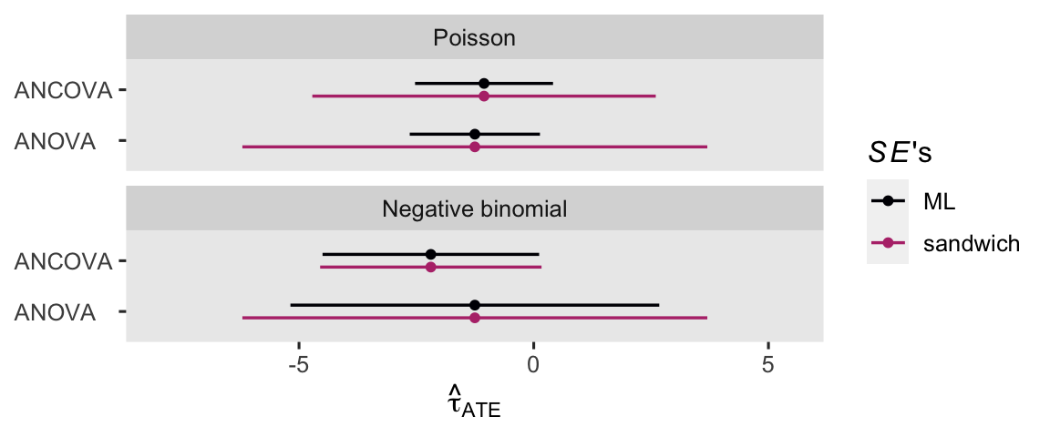
Broadly speaking, the ANCOVA models returned more precise estimates for \(\tau_\text{ATE}\). If you have high-quality baseline covariates laying around, put them to use!

Compute \(\lambda^1 - \lambda^0\) or \(\mu^1 - \mu^0\).

Within the context of our count models, it is still the case that

$$\tau_\text{ATE} = \mathbb E (y_i^1 - y_i^0) = \mathbb E (y_i^1) - \mathbb E (y_i^0).$$

Within the context of our Poisson ANOVA model

$$ \begin{align*} \mathbb E (y_i^1) & = \lambda^1,\ \text{and} \\ \mathbb E (y_i^0) & = \lambda^0, \end{align*} $$

which means

$$ \begin{align*} \tau_\text{ATE} = \mathbb E (y_i^1 - y_i^0) & = \mathbb E (y_i^1) - \mathbb E (y_i^0) \\ & = {\color{blueviolet}{\lambda^1 - \lambda^0}}. \end{align*} $$

In a similar way for our negative-binomial ANOVA model

$$ \begin{align*} \mathbb E (y_i^1) & = \mu^1,\ \text{and} \\ \mathbb E (y_i^0) & = \mu^0, \end{align*} $$

which means

$$ \begin{align*} \tau_\text{ATE} = \mathbb E (y_i^1 - y_i^0) & = \mathbb E (y_i^1) - \mathbb E (y_i^0) \\ & = {\color{blueviolet}{\mu^1 - \mu^0}}. \end{align*} $$

You can compute these predictions for either of the ANOVA models with base R predict(). But let’s just jump straight to the nicer marginaleffects::predictions() function. First we update our nd prediction grid, then we compute the estimates.

# simplify the prediction grid
nd <- tibble(Trt = factor(0:1))

# compute
predictions(fit1, newdata = nd, by = "Trt")

## 
##  Trt Estimate Pr(>|z|) 2.5 % 97.5 %
##    0     7.96   <0.001  6.98   9.08
##    1     6.71   <0.001  5.86   7.69
## 
## Columns: rowid, Trt, estimate, p.value, conf.low, conf.high, count

The first row is for the \(\hat \lambda^0\) value from the Poisson ANOVA, and the second row is for \(\hat \lambda^1\). In this case we used the conventional ML standard errors. One might also include vcov = "HC3" to use the sandwich standard errors, instead. To compute the predictions from the negative-binomial ANOVA, just switch out fit1 for fit2. To take the final step to compute the estimate for \(\tau_\text{ATE}\), just add hypothesis = "revpairwise".

predictions(fit1, newdata = nd, by = "Trt", hypothesis = "revpairwise")

## 
##   Term Estimate Std. Error     z Pr(>|z|) 2.5 % 97.5 %
##  1 - 0    -1.25      0.708 -1.77   0.0763 -2.64  0.133
## 
## Columns: term, estimate, std.error, statistic, p.value, conf.low, conf.high

For kicks and giggles, here’s a coefficient plot of \(\hat \tau_\text{ATE}\) from both versions of the ANOVA, with both kinds of standard errors.

bind_rows(
  predictions(fit1, newdata = nd, by = "Trt", hypothesis = "revpairwise"),
  predictions(fit1, newdata = nd, by = "Trt", hypothesis = "revpairwise", vcov = "HC3"),
  predictions(fit2, newdata = nd, by = "Trt", hypothesis = "revpairwise"),
  predictions(fit2, newdata = nd, by = "Trt", hypothesis = "revpairwise", vcov = "HC3")
) %>% 
  data.frame() %>% 
  mutate(se         = rep(ses, times = 2) %>% factor(., levels = ses),
         likelihood = rep(likelihoods, each = 2)) %>% 
  
  ggplot(aes(x = estimate, xmin = conf.low, xmax = conf.high, y = likelihood, color = se)) +
  geom_pointinterval(position = position_dodge(width = -0.5)) +
  scale_color_viridis_d(expression(italic(SE)*"'s"), option = "A", end = .5) +
  scale_x_continuous(expand = expansion(mult = 0.25)) +
  labs(x = expression(hat(tau)[ATE]),
       y = NULL) +
  theme(axis.text.y = element_text(hjust = 0))

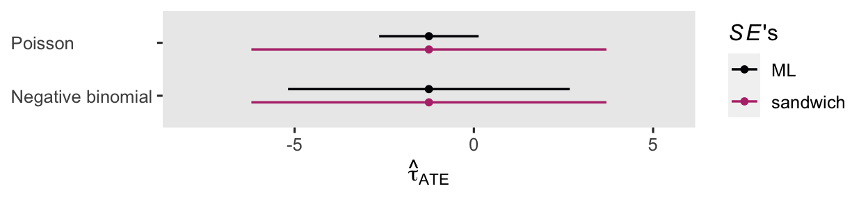
The point estimates are all the same, but the 95% intervals vary widely.

Do we compute \(\lambda^1 - \lambda^0\) or \(\mu^1 - \mu^0\) conditional on covariates?

As with the logistic regression context, we cannot use our Poisson or negative-binomial ANCOVA models to estimate \(\tau_\text{ATE}\) via the method we just explored, above. This is because for the Poisson and negative-binomial ANCOVA models,

$$ \tau_\text{CATE} = \operatorname{\mathbb{E}} (y_i^1 \mid \mathbf C = \mathbf c, \mathbf D = \mathbf d) - \operatorname{\mathbb{E}}(y_i^0 \mid \mathbf C = \mathbf c, \mathbf D = \mathbf d). $$

In words, when you subtract the counterfactual mean for the control condition from the counterfactual mean for the treatment condition, conditional on baseline covariate values, you get a conditional ATE (i.e., CATE), not the ATE. To my knowledge, there’s no way around this.

To express this equation in terms of the Poisson ANCOVA

$$\tau_\text{CATE} = ({\color{blueviolet}{\lambda^1}} \mid \mathbf C = \mathbf c, \mathbf D = \mathbf d) - ({\color{blueviolet}{\lambda^0}} \mid \mathbf C = \mathbf c, \mathbf D = \mathbf d),$$

and to express this equation in terms of the negative-binomial ANCOVA

$$\tau_\text{CATE} = ({\color{blueviolet}{\mu^1}} \mid \mathbf C = \mathbf c, \mathbf D = \mathbf d) - ({\color{blueviolet}{\mu^0}} \mid \mathbf C = \mathbf c, \mathbf D = \mathbf d).$$

As a consequence, you need to use the standardization/g-computation method if you want to estimate the ATE from a count ANCOVA model. But if you actually wanted a CATE, this method will work just fine. For example, way we wanted the CATE for a person with an average number of baseline seizure counts (about 23.4) and age (about 27.7), we would set both covariate values to zero and make the computation with predictions(). Here’s what that looks like for our Poisson ANCOVA model, using the sandwich standard errors.

# update the prediction grid
nd <- tibble(
  Trt    = factor(0:1),
  lcBase = 0,
  lcAge  = 0)

# conditional lambda's
predictions(fit3, newdata = nd, by = "Trt", vcov = "HC3")

## 
##  Trt Estimate Pr(>|z|) 2.5 % 97.5 % lcBase lcAge
##    0     5.34   <0.001  3.68   7.75      0     0
##    1     4.62   <0.001  3.51   6.09      0     0
## 
## Columns: rowid, Trt, estimate, p.value, conf.low, conf.high, lcBase, lcAge, count

# the CATE
predictions(fit3, newdata = nd, by = "Trt", vcov = "HC3", hypothesis = "revpairwise")

## 
##   Term Estimate Std. Error      z Pr(>|z|) 2.5 % 97.5 %
##  1 - 0    -0.72       1.34 -0.537    0.591 -3.35   1.91
## 
## Columns: term, estimate, std.error, statistic, p.value, conf.low, conf.high

For a CATE based on different covariate values, update the nd predictor grid as desired. The framework will work the same for either likelihood and whether you want ML- or sandwich-based standard errors. Just bear in mind that with Poisson and negative-binomial ANCOVA models using the conventional log link,

$$\tau_\text{ATE} \neq \tau_\text{CATE}.$$

You can compute the CATE if you want; just don’t confuse it with the ATE.

Bayesian models.

To save y’all from soul-crushing redundancy, I’m not going to repeat all the content from the frequentist models in the Bayesian section. Here we’ll explore some of the results with a Bayesian negative-binomial ANOVA and a Bayesian Poisson ANCOVA.

Define the equations and fit.

Our Bayesian negative-binomial ANOVA model will be of the form

$$ \begin{align*} \text{count}_i & \sim \operatorname{Negative Binomial}(\mu_i, \phi) \\ \log(\mu_i) & = \beta_0 + \beta_1 \text{Trt}_i \\ \beta_0 & \sim \operatorname{Normal}(\log(14), 1) \\ \beta_1 & \sim \operatorname{Normal}(0, 0.5) \\ \phi & \sim \operatorname{Gamma}(0.01, 0.01), \end{align*} $$

where the final three lines in the formula express the priors. By centering the prior for \(\beta_0\) on \(\log(14)\), I’m betting those in the control (placebo) condition will report about 1 seizure at day (i.e., 14 during the last 2-week period). But since I know very little about seizures, and even less about seizure medication trials, I’m very insure about that prior, which is why I’ve set the prior standard deviation to 1. In my experience, 1 on the log scale is pretty big. In case you’re not accustomed to how Gaussian priors on the log scale translate to counts on the natural scale, keep in mind that an exponentiated normal distribution is the same as the lognormal distribution of the same \(\mu\) and \(\sigma\) values. To give you a sense of what our \(\operatorname{Normal}(\log(14), 1)\) prior means on the count scale, we’ll plot with a little help from a few nice tidybayes functions. For the sake of comparison, we’ll take a look at the more confident \(\operatorname{Normal}(\log(14), 0.5)\) prior, too.

# log(14) is about 2.639057
c(prior(lognormal(2.639057, 0.5)),
  prior(lognormal(2.639057, 1))) %>% 
  parse_dist() %>% 
  
  ggplot(aes(y = prior, dist = .dist, args = .args)) +
  stat_halfeye(.width = c(.5, .95)) +
  scale_y_discrete(NULL, labels = str_c("lognormal(log(14), ", c(0.5, 1), ")"),
                   expand = expansion(add = 0.1)) +
  xlab(expression(exp(italic(p)(beta[0])))) +
  coord_cartesian(xlim = c(0, 120))

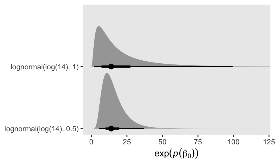
The dots mark the prior medians, and the thick and thinner horizontal lines mark the percentile-based 50% and 95% ranges, respectively. Even the seemingly specific \(\operatorname{Normal}(\log(14), 0.5)\) prior spreads the bulk of the prior mass around a decent portion of seizure count possibilities. But since I’m no expert in this domain, I’ve opted for the humbler \(\operatorname{Normal}(\log(14), 1)\) prior.

To my eye, a one-point difference on the log scale would be a pretty large treatment effect. So the \(\operatorname{Normal}(0, 0.5)\) prior for \(\beta_1\) is meant to protect against very large treatment effects for the experimental condition. Thus, it’s mildly conservative.

Finally, the \(\operatorname{Gamma}(0.01, 0.01)\) prior for \(\phi\) is the brms default. If you’re not familiar with setting priors for \(\phi\) I’d recommend you start here, and then build up some intuition after practicing with open data sets. Otherwise, keep in mind \(\phi\) can take on continuous positive values. Smaller values of \(\phi\) indicate larger overdispersion, and as \(\phi \rightarrow \infty\), the negative-binomial distribution converges with the Poisson. So based on our quick-and-dirty sample statistic analysis form above, I’d generally expect \(\phi\) values somewhere in the single-digit range, or maybe in the teens at the largest. But do keep in mind that basing your priors on sample statistics isn’t really kosher, since priors are supposed to express your expectations before (i.e., prior to) the data. But if you’re still a student and this is all new to you, go ahead and practice liberally. This is how we learn.

Our Bayesian Poisson ANCOVA model will be of the form

$$ \begin{align*} \text{count}_i & \sim \operatorname{Poisson}(\lambda_i) \\ \log(\lambda_i) & = \beta_0 + \beta_1 \text{Trt}_i + \beta_2 \text{lcBase}_i + \beta_3 \text{lcAge}_i \\ \beta_0 & \sim \operatorname{Normal}(\log(14), 1) \\ \beta_1 & \sim \operatorname{Normal}(0, 0.5) \\ \beta_2 & \sim \operatorname{Normal}(1, 0.5) \\ \beta_3 & \sim \operatorname{Normal}(0, 0.5), \end{align*} $$

where the priors for \(\beta_0\) and \(\beta_1\) are the same as in the previous model. However, because we’ve added the two baseline covariates, the \(\beta_0\) and \(\beta_1\) parameters are now conditional on the covariates at zero, which is their mean value back in their original metrics. To the extent those covariate values change how you think about \(\beta_0\) and \(\beta_1\), consider changing their priors accordingly.

I expect a strong positive correlation with the dependent variable and baseline counts (log-transformed and mean centered), and therefore the \(\operatorname{Normal}(1, 0.5)\) prior is designed to convey that expectation. My expectations are less certain for our dependent variable and age, and thus I defaulted to the more conservative and regularizing \(\operatorname{Normal}(0, 0.5)\).

Here are how to fit the two Bayesian models with the brm() function.

# NB ANOVA
brm1 <- brm(
  data = ep4,
  family = negbinomial,
  count ~ 0 + Intercept + Trt,
  prior = prior(normal(log(14), 1), class = b, coef = Intercept) +
    prior(normal(0, 0.5), class = b, coef = Trt1) +
    prior(gamma(0.01, 0.01), class = shape),
  cores = 4, seed = 5
)

# Poisson ANCOVA
brm2 <- brm(
  data = ep4,
  family = poisson,
  count ~ 0 + Intercept + Trt + lcBase + lcAge,
  prior = prior(normal(log(14), 1), class = b, coef = Intercept) +
    prior(normal(0, 0.5), class = b, coef = Trt1) +
    prior(normal(1, 0.5), class = b, coef = lcBase) +
    prior(normal(0, 0.5), class = b, coef = lcAge),
  cores = 4, seed = 5
)

Check the model summaries.

summary(brm1)

##  Family: negbinomial 
##   Links: mu = log; shape = identity 
## Formula: count ~ 0 + Intercept + Trt 
##    Data: ep4 (Number of observations: 59) 
##   Draws: 4 chains, each with iter = 2000; warmup = 1000; thin = 1;
##          total post-warmup draws = 4000
## 
## Population-Level Effects: 
##           Estimate Est.Error l-95% CI u-95% CI Rhat Bulk_ESS Tail_ESS
## Intercept     2.08      0.18     1.74     2.45 1.00     2313     2696
## Trt1         -0.14      0.24    -0.61     0.35 1.00     2391     2646
## 
## Family Specific Parameters: 
##       Estimate Est.Error l-95% CI u-95% CI Rhat Bulk_ESS Tail_ESS
## shape     1.04      0.22     0.66     1.52 1.00     2338     2358
## 
## Draws were sampled using sampling(NUTS). For each parameter, Bulk_ESS
## and Tail_ESS are effective sample size measures, and Rhat is the potential
## scale reduction factor on split chains (at convergence, Rhat = 1).

summary(brm2)

##  Family: poisson 
##   Links: mu = log 
## Formula: count ~ 0 + Intercept + Trt + lcBase + lcAge 
##    Data: ep4 (Number of observations: 59) 
##   Draws: 4 chains, each with iter = 2000; warmup = 1000; thin = 1;
##          total post-warmup draws = 4000
## 
## Population-Level Effects: 
##           Estimate Est.Error l-95% CI u-95% CI Rhat Bulk_ESS Tail_ESS
## Intercept     1.68      0.08     1.52     1.84 1.00     1870     2084
## Trt1         -0.15      0.10    -0.35     0.05 1.00     2267     2484
## lcBase        1.17      0.07     1.04     1.30 1.00     2344     2469
## lcAge         0.30      0.21    -0.11     0.70 1.00     2722     2621
## 
## Draws were sampled using sampling(NUTS). For each parameter, Bulk_ESS
## and Tail_ESS are effective sample size measures, and Rhat is the potential
## scale reduction factor on split chains (at convergence, Rhat = 1).

Both model summaries look fine, to me. If it wasn’t clear to you, the shape line near the bottom of the summary(brm1) output is for the \(\phi\) parameter.

Can the \(\beta\) posteriors give us the ATE?

I don’t want to spend a lot of time fooling with \(\beta\) posteriors themselves, in this post, but the overall framework applies much like it did for our frequentist models. We can compute the ATE from a count ANOVA model with the formula

$$\exp(\beta_0 + \beta_1) - \exp(\beta_0).$$

In our case, we’d pull the posteriors from each parameter with the as_draws_df() function, wrangle, and summarize as desired. Here’s what that can look like for our negative-binomial ANOVA brm1.

# wrangle
as_draws_df(brm1) %>% 
  mutate(`beta[0]` = b_Intercept,
         `beta[1]` = b_Trt1) %>% 
  # compute
  mutate(ate = exp(`beta[0]` + `beta[1]`) - exp(`beta[0]`)) %>% 
  # summarize
  mean_qi(ate)

## # A tibble: 1 × 6
##     ate .lower .upper .width .point .interval
##   <dbl>  <dbl>  <dbl>  <dbl> <chr>  <chr>    
## 1 -1.07  -4.93   2.64   0.95 mean   qi

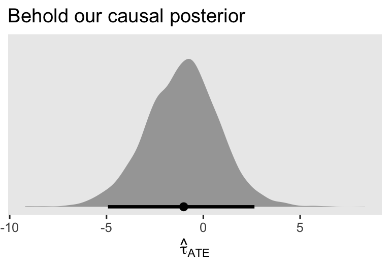
The first three columns displayed the posterior mean and percentile-based 95% interval for \(\hat \tau_\text{ATE}\). Just for kicks and giggles, here’s the whole distribution.

as_draws_df(brm1) %>% 
  mutate(`beta[0]` = b_Intercept,
         `beta[1]` = b_Trt1) %>% 
  mutate(ate = exp(`beta[0]` + `beta[1]`) - exp(`beta[0]`)) %>% 
  
  ggplot(aes(x = ate)) +
  stat_halfeye(.width = .95) +
  scale_y_continuous(NULL, breaks = NULL) +
  labs(title = "Behold our causal posterior",
       x = expression(hat(tau)[ATE]))

You cannot, however, compute the posterior for \(\tau_\text{ATE}\) based on the \(\beta\) posteriors from an ANCOVA version of this model. You need the standardization/g-computation method for that. Speaking of which…

Posteriors for \(\mathbb E (\lambda_i^1 - \lambda_i^0)\) and \(\mathbb E (\mu_i^1 - \mu_i^0)\).

With Bayes, it’s still the case that

$$\tau_\text{ATE} = \mathbb E (y_i^1 - y_i^0),$$

even with your count models. But as we learned in the last post, applied Bayesian inference via MCMC methods adds a new procedural complication for the \(\mathbb E (y_i^1 - y_i^0)\) method. If you let \(j\) stand for a given MCMC draw, we end up computing

$$\tau_{\text{ATE}_j} = \mathbb E_j (y_{ij}^1 - y_{ij}^0), \ \text{for}\ j = 1, \dots, J,$$

which in words means we compute the familiar \(\mathbb E (y_i^1 - y_i^0)\) for each of the \(J\) MCMC draws. This returns a \(J\)-row vector for the \(\tau_\text{ATE}\) distribution, which we can then summarize the same as we would any other dimension of the posterior distribution. And since we’re working with count models, we might rewrite this as

$$\tau_{\text{ATE}_j} = \mathbb E_j ({\color{blueviolet}{\lambda}}_{ij}^1 - {\color{blueviolet}{\lambda}}_{ij}^0), \ \text{for}\ j = 1, \dots, J,$$

for a Poisson model, and

$$\tau_{\text{ATE}_j} = \mathbb E_j ({\color{blueviolet}{\mu}}_{ij}^1 - {\color{blueviolet}{\mu}}_{ij}^0), \ \text{for}\ j = 1, \dots, J,$$

for a negative-binomial model. In our last post, we practiced computing such quantities with three methods:

• a fitted()-based approach,
• an as_draws_df()-based approach, and
• a predictions()/avg_comparisons()-based approach.

We’ll do the same thing here.

As a first step, let’s make our summarization tasks easier by making a custom summarizing function I like to call brms_summary().

brms_summary <- function(x) {
  posterior::summarise_draws(x, "mean", "sd",  ~quantile(.x, probs = c(0.025, 0.975)))
}

You, of course, could also use something like summarise() or median_qi(), instead. Next, we update our nd predictor grid.

nd <- ep4 %>% 
  select(patient, lcBase, lcAge) %>% 
  expand_grid(Trt = factor(0:1)) %>% 
  mutate(row = 1:n())

# what?
glimpse(nd)

## Rows: 118
## Columns: 5
## $ patient <fct> 1, 1, 2, 2, 3, 3, 4, 4, 5, 5, 6, 6, 7, 7, 8, 8, 9, 9, 10, 10, 11, 11, 12, 12, 13, 13, 14, 14…
## $ lcBase  <dbl> -0.75635379, -0.75635379, -0.75635379, -0.75635379, -1.36248959, -1.36248959, -1.07480752, -…
## $ lcAge   <dbl> 0.11420370, 0.11420370, 0.08141387, 0.08141387, -0.10090768, -0.10090768, 0.26373543, 0.2637…
## $ Trt     <fct> 0, 1, 0, 1, 0, 1, 0, 1, 0, 1, 0, 1, 0, 1, 0, 1, 0, 1, 0, 1, 0, 1, 0, 1, 0, 1, 0, 1, 0, 1, 0,…
## $ row     <int> 1, 2, 3, 4, 5, 6, 7, 8, 9, 10, 11, 12, 13, 14, 15, 16, 17, 18, 19, 20, 21, 22, 23, 24, 25, 2…

Notice that unlike what we’ve done before, we added a row index. This will help us join our nd data to the fitted() output, below. Speaking of which, here’s the posterior summary for the ATE, based on our Bayesian negative-binomial ANOVA.

fitted(brm1,
       newdata = nd,
       summary = F) %>% 
  data.frame() %>% 
  set_names(pull(nd, row)) %>% 
  mutate(draw = 1:n()) %>% 
  pivot_longer(-draw) %>% 
  mutate(row = as.double(name)) %>% 
  left_join(nd, by = "row") %>% 
  select(draw, value, patient, Trt) %>% 
  pivot_wider(names_from = Trt, values_from = value) %>% 
  mutate(tau = `1` - `0`) %>% 
  # first compute the ATE within each MCMC draw
  group_by(draw) %>% 
  summarise(ate = mean(tau)) %>% 
  select(ate) %>% 
  # now summarize the ATE across the MCMC draws
  brms_summary()

## # A tibble: 1 × 5
##   variable  mean    sd `2.5%` `97.5%`
##   <chr>    <num> <num>  <num>   <num>
## 1 ate      -1.07  1.90  -4.93    2.64

Here’s the add_epred_draws() alternative.

nd %>% 
  add_epred_draws(brm1) %>% 
  ungroup() %>%
  select(Trt, patient, .draw, .epred) %>% 
  pivot_wider(names_from = Trt, values_from = .epred) %>% 
  mutate(tau = `1` - `0`) %>% 
  # first compute the ATE within each MCMC draw
  group_by(.draw) %>% 
  summarise(ate = mean(tau)) %>% 
  select(ate) %>% 
  # now summarize the ATE across the MCMC draws
  brms_summary()

## # A tibble: 1 × 5
##   variable  mean    sd `2.5%` `97.5%`
##   <chr>    <num> <num>  <num>   <num>
## 1 ate      -1.07  1.90  -4.93    2.64

Here’s the marginaleffects::avg_comparisons() approach.

# change the **marginaleffects** default to use the mean
options(marginaleffects_posterior_center = mean)

# now summarize the ATE across the MCMC draws
avg_comparisons(brm1, variables = list(Trt = 0:1))

## 
##  Term Contrast Estimate 2.5 % 97.5 %
##   Trt    1 - 0    -1.07 -4.93   2.64
## 
## Columns: term, contrast, estimate, conf.low, conf.high

Whether you prefer a fitted()-, as_draws_df()-, or avg_comparisons()-based workflow, this is all just standardization/g-computation methodology as applied to MCMC-based Bayesian models. This process works exactly the same if you’d like to instead use the standardization/g-computation approach for a Bayesian count ANCOVA model. As a quick example, here’s the add_epred_draws()-based code for our Bayesian Poisson ANCOVA brm2.

nd %>% 
  add_epred_draws(brm2) %>% 
  ungroup() %>%
  select(Trt, patient, .draw, .epred) %>% 
  pivot_wider(names_from = Trt, values_from = .epred) %>% 
  mutate(tau = `1` - `0`) %>% 
  # first compute the ATE within each MCMC draw
  group_by(.draw) %>% 
  summarise(ate = mean(tau)) %>% 
  select(ate) %>% 
  # now summarize the ATE across the MCMC draws
  brms_summary()

## # A tibble: 1 × 5
##   variable  mean    sd `2.5%` `97.5%`
##   <chr>    <num> <num>  <num>   <num>
## 1 ate      -1.13 0.730  -2.55   0.335

I’ll leave it up to the interested reader to practice the same with a fitted() or avg_comparisons() workflow. They’ll all return the same results.

Posteriors for \(\lambda^1 - \lambda^0\) and \(\mu^1 - \mu^0\).

As with the frequentist framework, we can only compute our posteriors for the ATE with the group-mean difference method with the ANOVA versions of the Bayesian count models. Within the context of our negative-binomial brm1, that means

$$ \begin{align*} \tau_\text{ATE} = \mathbb E (y_i^1 - y_i^0) & = \mathbb E (y_i^1) - \mathbb E (y_i^0) \\ & = {\color{blueviolet}{\mu^1 - \mu^0}}. \end{align*} $$

Here’s what that looks like with a fitted()-based workflow.

nd <- tibble(Trt = factor(0:1))

fitted(brm1,
       newdata = nd,
       summary = F) %>% 
  data.frame() %>% 
  set_names(pull(nd, Trt)) %>% 
  mutate(ate = `1` - `0`) %>% 
  brms_summary()

## # A tibble: 3 × 5
##   variable  mean    sd `2.5%` `97.5%`
##   <chr>    <num> <num>  <num>   <num>
## 1 0         8.15  1.53   5.67   11.6 
## 2 1         7.08  1.35   4.91   10.2 
## 3 ate      -1.07  1.90  -4.93    2.64

The top two rows are the posterior summaries for \(\mu^0\) and \(\mu^1\), and the third row is their contrast, the ATE. Here’s the same via the add_epred_draws() method.

nd %>% 
  add_epred_draws(brm1) %>% 
  ungroup() %>%
  select(Trt, .draw, .epred) %>% 
  pivot_wider(names_from = Trt, values_from = .epred)  %>% 
  mutate(ate = `1` - `0`) %>% 
  brms_summary()

## # A tibble: 3 × 5
##   variable  mean    sd `2.5%` `97.5%`
##   <chr>    <num> <num>  <num>   <num>
## 1 0         8.15  1.53   5.67   11.6 
## 2 1         7.08  1.35   4.91   10.2 
## 3 ate      -1.07  1.90  -4.93    2.64

Now we practice with the predictions() method.

# predicted mu's
predictions(brm1, newdata = nd, by = "Trt")

## 
##  Trt Estimate 2.5 % 97.5 %
##    0     8.15  5.67   11.6
##    1     7.08  4.91   10.2
## 
## Columns: rowid, Trt, estimate, conf.low, conf.high, count

# ATE
predictions(brm1, newdata = nd, by = "Trt", hypothesis = "revpairwise")

## 
##   Term Estimate 2.5 % 97.5 %
##  1 - 0    -1.07 -4.93   2.64
## 
## Columns: term, estimate, conf.low, conf.high

Do we compute the Bayesian \(\lambda^1 - \lambda^0\) or \(\mu^1 - \mu^0\) conditional on covariates?

As with our frequentist count models, we can’t use the group-mean-contrast method to compute the ATE from a count ANCOVA. The best we can do with this method is compute a CATE. Here are the conditional \(\lambda\)’s and their contrast for a person with a mean baseline siezure count and mean age, using the thrifty predictions() method.

# update the prediction grid
nd <- tibble(
  Trt    = factor(0:1),
  lcBase = 0,
  lcAge  = 0)

# conditional lambda's
predictions(brm2, newdata = nd, by = "Trt")

## 
##  Trt Estimate 2.5 % 97.5 % lcBase lcAge
##    0     5.40  4.57   6.31      0     0
##    1     4.62  3.92   5.40      0     0
## 
## Columns: rowid, Trt, estimate, conf.low, conf.high, lcBase, lcAge, count

# the CATE
predictions(brm2, newdata = nd, by = "Trt", hypothesis = "revpairwise")

## 
##   Term Estimate 2.5 % 97.5 %
##  1 - 0   -0.772 -1.74  0.226
## 
## Columns: term, estimate, conf.low, conf.high

I’ll leave it up to the interested reader to practice the same with a fitted() or add_epred_draws() workflow. Though our code here used our Bayesian Poisson ANCOVA, it would have worked the same way with a Bayesian negative-binomial ANCOVA.

Lingering issues

What about those “robust” SE’s for Bayesian models?

The whole robust sandwich standard error issue mainly applies to frequentist models. Some are starting to propose similar methods for Bayesian models (e.g., Szpiro et al., 2010), but I am not aware those solutions are available with brms (see this discussion). If you don’t like the assumptions inherent in your likelihood function, think hard about alternative likelihoods. If you’re aware of another Bayesian alternative, tell me all about it in the comments section, below.

Can we trust the negative binomial?

There’s some concern over whether the negative-binomial model can show bias under certain conditions, which leads into a technical issue I’ve avoided up until this point. There are two major ways to parameterize the negative-binomial model. The canonical version is often called NB1, and the more popular version is called NB2. For a nice historical overview on the two versions, see Chapter 1 in Hilbe ( 2011). Whether with the MASS::glm.nb() function or the brms::brm() function, all the negative-binomial models in this blog post used the NB2 parameterization. In a nice simulation study, Blackburn ( 2015) showed the NB1 approach can return markedly biased \(\beta\) coefficients when the variance in the sample data doesn’t perfectly match the model. The NB2 approach can show parameter bias in some conditions, but the magnitude of the bias was generally pretty small (to my eye), and it performed pretty well overall. These kinds of concerns have led some to prefer so-called quasi-likelihood approaches, which are not to my taste and will not be further explored in this blog series. But if you’re curious, you can learn about quasi-likelihood approaches in Chapter 9 of McCullagh & Nelder ( 1989).

I’d like to thank the great Noah Greifer for dragging me kicking and screaming into this topic.

Recap

In this post, some of the main points we covered were:

• With count regression, the \(\beta_1\) coefficient has no direct relationship with the ATE, regardless of whether you have included covariates.
• For the Poisson regression ANOVA model,
  • \(\tau_\text{ATE} = \mathbb E (\lambda_i^1 - \lambda_i^0)\), and
  • \(\tau_\text{ATE} = \lambda^1 - \lambda^0\).
• For the negative-binomial ANOVA model,
  • \(\tau_\text{ATE} = \mathbb E (\mu_i^1 - \mu_i^0)\), and
  • \(\tau_\text{ATE} = \mu^1 - \mu^0\).
• For the Poisson regression ACNOVA model,
  • \(\tau_\text{ATE} = \mathbb E (\lambda_i^1 - \lambda_i^0 \mid \mathbf C_i, \mathbf D_i)\), but
  • \(\tau_\text{CATE} = (\lambda^1 \mid \mathbf C = \mathbf c, \mathbf D = \mathbf d) - (\lambda^0 \mid \mathbf C = \mathbf c, \mathbf D = \mathbf d)\).
• For the negative-binomial ACNOVA model,
  • \(\tau_\text{ATE} = \mathbb E (\mu_i^1 - \mu_i^0 \mid \mathbf C_i, \mathbf D_i)\), but
  • \(\tau_\text{CATE} = (\mu^1 \mid \mathbf C = \mathbf c, \mathbf D = \mathbf d) - (\mu^0 \mid \mathbf C = \mathbf c, \mathbf D = \mathbf d)\).
• For Poisson or negative-binomial ANCOVA models, there can be many different values for the conditional average treatment effect, \(\tau_\text{CATE}\), depending which values one uses for the covariates.
• Sometimes frequentists prefer sandwich standard errors over the conventional ML standard errors for their count models. For Bayesians, the posterior \(\textit{SD}\) is just the posterior \(\textit{SD}\). If you don’t like it, think harder about your likelihood.

In the next post, we’ll explore how our causal inference methods work with gamma regression models.

Thank the reviewer

I’d like to publicly acknowledge and thank

• Stephen J. Wild

for his kind efforts reviewing the draft of this post. Go team!

Do note the final editorial decisions were my own, and I do not think it would be reasonable to assume my reviewer has given a blanket endorsement of the current version of this post.

Session info

sessionInfo()

## R version 4.2.3 (2023-03-15)
## Platform: x86_64-apple-darwin17.0 (64-bit)
## Running under: macOS Big Sur ... 10.16
## 
## Matrix products: default
## BLAS:   /Library/Frameworks/R.framework/Versions/4.2/Resources/lib/libRblas.0.dylib
## LAPACK: /Library/Frameworks/R.framework/Versions/4.2/Resources/lib/libRlapack.dylib
## 
## locale:
## [1] en_US.UTF-8/en_US.UTF-8/en_US.UTF-8/C/en_US.UTF-8/en_US.UTF-8
## 
## attached base packages:
## [1] stats     graphics  grDevices utils     datasets  methods   base     
## 
## other attached packages:
##  [1] patchwork_1.1.2             marginaleffects_0.11.1.9008 tidybayes_3.0.4            
##  [4] sandwich_3.0-2              lmtest_0.9-40               zoo_1.8-10                 
##  [7] ggdist_3.2.1.9000           broom_1.0.4                 GGally_2.1.2               
## [10] flextable_0.9.1             brms_2.19.0                 Rcpp_1.0.10                
## [13] lubridate_1.9.2             forcats_1.0.0               stringr_1.5.0              
## [16] dplyr_1.1.2                 purrr_1.0.1                 readr_2.1.4                
## [19] tidyr_1.3.0                 tibble_3.2.1                ggplot2_3.4.2              
## [22] tidyverse_2.0.0            
## 
## loaded via a namespace (and not attached):
##   [1] uuid_1.1-0              backports_1.4.1         systemfonts_1.0.4       plyr_1.8.7             
##   [5] igraph_1.3.4            svUnit_1.0.6            splines_4.2.3           crosstalk_1.2.0        
##   [9] katex_1.4.0             TH.data_1.1-1           rstantools_2.2.0        inline_0.3.19          
##  [13] digest_0.6.31           htmltools_0.5.5         fansi_1.0.4             magrittr_2.0.3         
##  [17] checkmate_2.1.0         tzdb_0.3.0              RcppParallel_5.1.5      matrixStats_0.63.0     
##  [21] xslt_1.4.3              officer_0.6.2           xts_0.12.1              askpass_1.1            
##  [25] timechange_0.2.0        gfonts_0.2.0            prettyunits_1.1.1       colorspace_2.1-0       
##  [29] textshaping_0.3.6       xfun_0.39               callr_3.7.3             crayon_1.5.2           
##  [33] jsonlite_1.8.4          lme4_1.1-31             survival_3.5-3          glue_1.6.2             
##  [37] gtable_0.3.3            emmeans_1.8.0           V8_4.2.1                distributional_0.3.1   
##  [41] pkgbuild_1.3.1          rstan_2.21.8            abind_1.4-5             scales_1.2.1           
##  [45] fontquiver_0.2.1        mvtnorm_1.1-3           DBI_1.1.3               miniUI_0.1.1.1         
##  [49] viridisLite_0.4.1       xtable_1.8-4            stats4_4.2.3            StanHeaders_2.21.0-7   
##  [53] fontLiberation_0.1.0    DT_0.24                 collapse_1.9.2          htmlwidgets_1.5.4      
##  [57] threejs_0.3.3           arrayhelpers_1.1-0      RColorBrewer_1.1-3      posterior_1.4.1        
##  [61] ellipsis_0.3.2          reshape_0.8.9           pkgconfig_2.0.3         loo_2.5.1              
##  [65] farver_2.1.1            sass_0.4.5              crul_1.2.0              utf8_1.2.3             
##  [69] labeling_0.4.2          tidyselect_1.2.0        rlang_1.1.0             reshape2_1.4.4         
##  [73] later_1.3.0             munsell_0.5.0           tools_4.2.3             cachem_1.0.7           
##  [77] cli_3.6.1               generics_0.1.3          evaluate_0.20           fastmap_1.1.1          
##  [81] ragg_1.2.5              yaml_2.3.7              processx_3.8.1          knitr_1.42             
##  [85] zip_2.2.0               nlme_3.1-162            equatags_0.2.0          mime_0.12              
##  [89] projpred_2.2.1          xml2_1.3.3              compiler_4.2.3          bayesplot_1.10.0       
##  [93] shinythemes_1.2.0       rstudioapi_0.14         gamm4_0.2-6             curl_5.0.0             
##  [97] bslib_0.4.2             stringi_1.7.12          highr_0.10              ps_1.7.5               
## [101] blogdown_1.16           Brobdingnag_1.2-8       gdtools_0.3.3           lattice_0.20-45        
## [105] Matrix_1.5-3            fontBitstreamVera_0.1.1 nloptr_2.0.3            markdown_1.1           
## [109] shinyjs_2.1.0           tensorA_0.36.2          vctrs_0.6.2             pillar_1.9.0           
## [113] lifecycle_1.0.3         jquerylib_0.1.4         bridgesampling_1.1-2    estimability_1.4.1     
## [117] insight_0.19.1.6        data.table_1.14.8       httpuv_1.6.5            R6_2.5.1               
## [121] bookdown_0.28           promises_1.2.0.1        gridExtra_2.3           codetools_0.2-19       
## [125] boot_1.3-28.1           colourpicker_1.1.1      MASS_7.3-58.2           gtools_3.9.4           
## [129] openssl_2.0.6           httpcode_0.3.0          withr_2.5.0             shinystan_2.6.0        
## [133] multcomp_1.4-20         mgcv_1.8-42             parallel_4.2.3          hms_1.1.3              
## [137] grid_4.2.3              coda_0.19-4             minqa_1.2.5             rmarkdown_2.21         
## [141] shiny_1.7.2             base64enc_0.1-3         dygraphs_1.1.1.6

References

Blackburn, M. L. (2015). The relative performance of Poisson and negative binomial regression estimators. Oxford Bulletin of Economics and Statistics, 77(4), 605–616. https://doi.org/10.1111/obes.12074
Greene, W. H. (2018). Econometric analysis (Eighth Edition). Pearson.
Hilbe, J. M. (2011). Negative binomial regression (Second Edition). https://doi.org/10.1017/CBO9780511973420
Hothorn, T., Zeileis, A., Farebrother, R. W., & Cummins, C. (2022). Lmtest: Testing Linear Regression Models. https://CRAN.R-project.org/package=lmtest
Leppik, I., Dreifuss, F., Bowman-Cloyd, T., Santilli, N., Jacobs, M., Crosby, C., Cloyd, J., Stockman, J., Graves, N., Sutula, T., et al. (1985). A double-blind crossover evaluation of progabide in partial seizures. Neurology, 35(4), 285–295.
McCullagh, P., & Nelder, J. A. (1989). Generalized linear models (Second Edition). Chapman and Hall.
Ripley, B. (2022). MASS: Support functions and datasets for venables and Ripley’s MASS. https://CRAN.R-project.org/package=MASS
Schloerke, B., Crowley, J., Di Cook, Briatte, F., Marbach, M., Thoen, E., Elberg, A., & Larmarange, J. (2021). GGally: Extension to ’ggplot2’. https://CRAN.R-project.org/package=GGally
Szpiro, A. A., Rice, K. M., & Lumley, T. (2010). Model-robust regression and a Bayesian “sandwich” estimator. Annals of Applied Statistics, 4(4), 2099–2113. https://doi.org/10.1214/10-AOAS362
Thall, P. F., & Vail, S. C. (1990). Some covariance models for longitudinal count data with overdispersion. Biometrics, 46(3), 657–671. https://doi.org/10.2307/2532086
Venables, W. N., & Ripley, B. D. (2002). Modern applied statistics with S (Fourth Edition). Springer. http://www.stats.ox.ac.uk/pub/MASS4
Zeileis, A. (2004). Econometric computing with HC and HAC covariance matrix estimators. Journal of Statistical Software, 11(10), 1–17. https://doi.org/10.18637/jss.v011.i10
Zeileis, A. (2006). Object-oriented computation of sandwich estimators. Journal of Statistical Software, 16(9), 1–16. https://doi.org/10.18637/jss.v016.i09
Zeileis, A., & Hothorn, T. (2002). Diagnostic Checking in Regression Relationships. R News, 2(3), 7–10. https://CRAN.R-project.org/doc/Rnews/
Zeileis, A., Köll, S., & Graham, N. (2020). Various versatile variances: An object-oriented implementation of clustered covariances in R. Journal of Statistical Software, 95(1), 1–36. https://doi.org/10.18637/jss.v095.i01
Zeileis, A., & Lumley, T. (2022). Sandwich: Robust covariance matrix estimators [Manual]. https://sandwich.R-Forge.R-project.org/
-
I haven’t been able to locate the actual paper by Leppik et al. ( 1985). If you have a copy, I’d love to see it. ↩︎
For ideas on what that might look like, execute
?epilepsyand scroll down to the bottom of the help page. ↩︎ -
Careful readers will note those sample statistics end up closer to the medians, rather than the means, of the original un-transformed variables. Logs are tricky, friends. ↩︎
Okay, technically you can have a censored or truncated count, which complicates how you think about the lower limit. In this post, we’re not focusing on those issues. Thus, our lower limit is the conventional value zero. But if you ever find yourself in a position where you have to contend with those issues, brms can handle both censored and truncated data. ↩︎
Clever readers will note our quick-and-dirty sample-statistic analysis is a lot like checking for equidispersion without controlling for the baseline covariates
BaseandAge. Maybe it’d be okay to presume equidispersion after conditioning on the baseline covariates. See how tricky this all gets? ↩︎
- Posted on:
- May 7, 2023
- Length:
- 47 minute read, 9879 words