Set your sigma prior when you know very little about your sum-score data

What?

We psychologists analyze a lot of sum-score data. Even though it’s not the best, we usually use the Gaussian likelihood¹ for these analyses. I was recently in a situation were I wanted to model sum-scores from a new questionnaire and there was no good prior research on the distribution of the sum-scores. Like, there wasn’t a single published paper reporting the sample statistics. Crazy, I know… Anyway, I spent some time trying to reason through how I would set a justifiable prior for my \(\sigma\) parameter, and in this blog post we’ll cover how I came up with a solution.

I make assumptions.

• For this post, I’m presuming you are familiar with Bayesian regression. For an introduction, I recommend either edition of McElreath’s text ( 2020, 2015); Kruschke’s ( 2015) text; or Gelman, Hill, and Vehtari’s ( 2020) text.

• All code is in R. Data wrangling and plotting were done with help from the tidyverse ( Wickham et al., 2019; Wickham, 2022), tidybayes ( Kay, 2022), and patchwork ( Pedersen, 2022). The Bayesian model will be fit with brms ( Bürkner, 2017, 2018, 2022). We will also use the MetBrewer package ( Mills, 2022) to select the color palette for our figures.

Here we load the packages and adjust the global plotting theme.

# load
library(tidyverse)
library(tidybayes)
library(patchwork)
library(brms)
library(MetBrewer)

# save a color vector
h <- met.brewer(colorblind_palettes[8])  # "Hiroshige"

# adjust the global plotting theme
theme_set(
  theme_linedraw(base_size = 13) +
    theme(panel.background = element_rect(fill = alpha(h[5], 0.33)),
          panel.border = element_rect(linewidth = 0.33),
          panel.grid = element_blank(),
          plot.background = element_rect(fill = alpha(h[5], 0.2)),
          strip.background = element_rect(fill = alpha(h[5], 0.67), linewidth = 0),
          strip.text = element_text(color = "black"))
)

The color palette in this post is inspired by Utagawa Hiroshige’s Sailing Boats Returning to Yabase, Lake Biwa, about which you can learn more from The Met’s website.

Overview

I came up with three broad strategies for settling in on a prior for \(\sigma\) when in a state of relative ignorance:

• Compute the maximum value with Popoviciu’s inequality.
• Compute an approximate standard deviation presuming a uniform distribution.
• Compute standard deviations based on plausible beta-binomial distributions.

We’ll explore each in turn.

Popoviciu’s inequality.

If you have continuous data with clear lower and upper boundaries, you can use Popoviciu’s ( 1935) inequality on variances to compute the maximum variance of the distribution. If we let \(U\) be the upper bound and \(L\) be the lower bound, Popoviciu’s inequality states

$$ \sigma^2 \leq \frac{1}{4} (U - L)^2. $$

For example, let’s say you’re using a questionnaire like the PHQ-9 ( Spitzer et al., 1999), which is a widely-used depression questionnaire² composed of 9 Likert-type items ranging from 0 to 3. The PHQ-9 sum score has a possible range of 0 to 27, with higher scores indicating deeper depression. Using Popoviciu’s inequality, we can compute the maximum variance for the PHQ-9 sum score like so.

u <- 27  # upper limit
l <- 0   # lower limit

(u - l)^2 / 4  # maximum variance

## [1] 182.25

Since variances are the same as standard deviations squared, we can take the square root of that value to compute the maximum standard deviation possible for the PHQ-9.

sqrt((u - l)^2 / 4)  # maximum standard deviation

## [1] 13.5

We might check this out with a little simulation. If we had a data set composed of \(N = 10{,}000\) PHQ-9 sum-score values which were evenly split between all zero’s and all 27’s, here’s what the sample standard deviation would be.

n <- 10000

tibble(y = rep(c(0, 27), each = n / 2)) %>% 
  summarise(var = var(y),
            sd = sd(y))

## # A tibble: 1 × 2
##     var    sd
##   <dbl> <dbl>
## 1  182.  13.5

The displayed output values are rounded, but the sample statistics are just a hair above the population values from Popoviciu’s inequality³.

When in a state of complete ignorance, you know your \(\sigma\) prior should be centered somewhere between zero and the value returned by Popoviciu’s inequality. Though I wouldn’t recommend it, one way to use this information would be to set a uniform prior ranging from zero to the upper-limit based on Popoviciu’s inequality.

Take the standard deviation from the uniform distribution.

Though Popoviciu’s inequality gives us a sense of the range of possible values, it doesn’t do a great job helping us decide which parts of that range are more likely than not. As a next stab, you might assume the sum-score data were uniformly distributed. This would be something of a null hypothesis stating: All values are equally likely.

If you have a uniform distribution with a lower limit of \(L\) and an upper limit of \(U\), you can compute the variance with the equation

$$ \sigma^2 = \frac{1}{12} (U - L)^2, $$

with the standard deviation being the square root of that value. Continuing on with our PHQ-9 data as an example, here are the variance and standard deviation presuming they were uniformly distributed.

u <- 27  # upper limit
l <- 0   # lower limit

(u - l)^2 / 12  # variance

## [1] 60.75

sqrt((u - l)^2 / 12)  # sd

## [1] 7.794229

Again, let’s run a little simulation to see how this shakes out.

n_option <- 1000

tibble(y = rep(0:27, each = n_option)) %>% 
  summarise(var = var(y),
            sd = sd(y))

## # A tibble: 1 × 2
##     var    sd
##   <dbl> <dbl>
## 1  65.3  8.08

In this case, the sample statistics from our simulation are a little bit off from the statistics we’d expect based on the formula from the uniform distribution. Here, though, keep in mind that the uniform distribution presumes truly continuous data, not integer values like those you’d get from a sum score. Thus the uniform distribution is only an approximation, not a true analogue. However, this isn’t a bad approach if you just want to get a sense of where to start.

Thus Popoviciu’s inequality gave us a possible range for \(\sigma\), and the uniform distribution gave us an approximate value given the null assumption all sum-scores are equally plausible.

But do you really want to use the null assumption that all sum-scores are equally plausible? If not, we’ll want to work with a new distribution.

Sum scores might look beta-binomial.

So even though we tend to use the Gaussian likelihood to model sum-score data for reasons⁴, it’s not the only distribution in town. If you search around in the backwater of applied statistics, you’ll find papers on the beta-binomial likelihood for sum-score-type data. For example, Lord discussed the beta-binomial distribution for psychological test data in ( 1962), Wilcox later reviewed it for the same purpose in ( 1981), and Carlin and Rubin kept the conversation rolling in ( 1991). Though these authors didn’t focus on Likert-type data per se, Greenleaf used the beta-binomial to describe a distribution of sums of Likert-type items in ( 1992). I’d like to extrapolate further and suggest the beta-binomial distribution can help us understand sum-score data in general, and the standard deviations of sum-score data in particular.

Given some count variable \(y\) with a clear upper bound \(n\), we can describe the beta-binomial likelihood as

$$ f(y | n, \alpha, \beta) = \binom{n}{y} \frac{\operatorname B (y + \alpha, n - y + \beta)}{\operatorname B(\alpha, \beta)}, $$

where \(\alpha\) and \(\beta\) are the two parameters from the canonical version of the beta likelihood, \(\operatorname B(\cdot)\) is the beta function, and \(\tbinom{n}{y}\) is a shorthand factorial notation. The \(\alpha\) and \(\beta\) parameters aren’t the most intuitive, but for our purposes the main thing to understand is when the mean of the distribution is in the middle of the range, \(\alpha = \beta\). I propose that when you are in a state of ignorance about a new sum-score, your go-to assumption should be the mean is in the middle. Why? Well, you have to start somewhere and the middle is at least as good a place as any other. But also keep in mind that most questionnaire developers have had at least some⁵ training in psychometrics, and they know that it’s generally a good idea to develop measures with approximately bell-shaped and symmetric distributions. Thus even of you’ve never seen prior examples of a given sum score, a good initial guess is the sample mean is somewhere in the middle of the possible range.

In the case of our PHQ-9 example where the lower limit is zero and the upper limit is 27, we could presume the data were uniformly distributed with \(\operatorname{BetaBinomial}(27, 1, 1)\). We can simulate data of that kind with the rbetabinom.ab() function from the VGAM package ( Yee, 2022). Here’s a sample of \(N = 10{,}000\).

set.seed(9)

d <- tibble(phq = VGAM::rbetabinom.ab(n = 1e4, size = 27, shape1 = 1, shape2 = 1))

# what?
head(d)

## # A tibble: 6 × 1
##     phq
##   <dbl>
## 1    20
## 2    23
## 3    16
## 4    17
## 5    10
## 6    22

Here’s what our simulated phq values look like in a plot.

d %>% 
  ggplot(aes(x = phq)) +
  geom_bar(fill = h[7]) +
  scale_x_continuous(breaks = 0:3 * 9) +
  ggtitle("10,000 draws from BetaBinomial(27, 1, 1)")

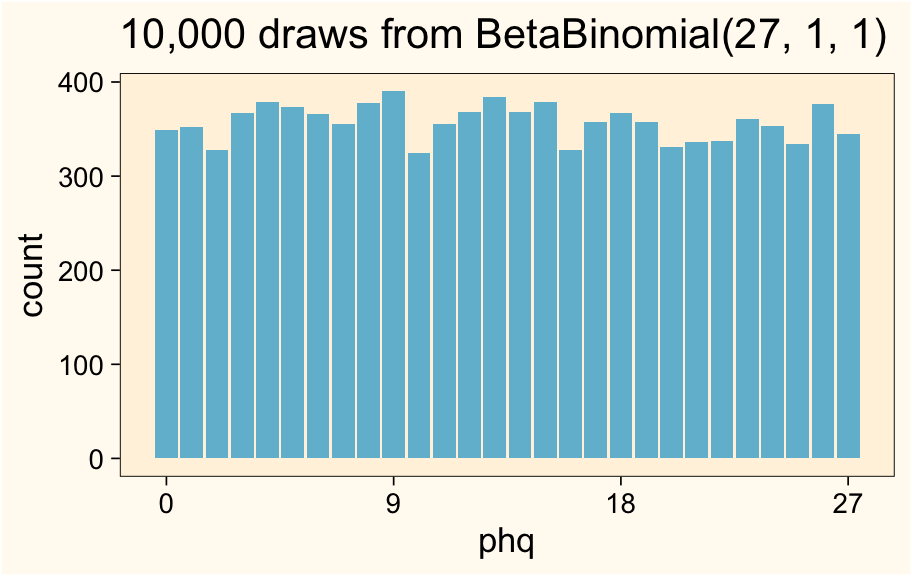
Here are the sample statistics.

d %>% 
  summarise(m = mean(phq),
            v = var(phq),
            s = sd(phq))

## # A tibble: 1 × 3
##       m     v     s
##   <dbl> <dbl> <dbl>
## 1  13.4  64.6  8.04

Now we’ve shifted from the exponential distribution to the beta-binomial, we might point out the variance of the beta-binomial is defined as

$$ \sigma^2 = \frac{n \alpha \beta (\alpha + \beta + n)}{(\alpha + \beta)^2 (\alpha + \beta + 1)}, $$

and the standard deviation of the beta-binomial is just the square root of that value. Here’s what that looks like in the case of \(\operatorname{BetaBinomial}(27, 1, 1)\).

n <- 27
a <- 1
b <- a

# population variance
((n * a * b) * (a + b + n)) / ((a + b)^2 * (a + b + 1))

## [1] 65.25

# population sd
sqrt(((n * a * b) * (a + b + n)) / ((a + b)^2 * (a + b + 1)))

## [1] 8.077747

So if we’re willing to describe the sum scores of our Likert-type items as integers, the flat beta-binomial may give us a better first stab at the standard deviation than the exponential distribution approach, above.

But we can go further. The beta-binomial \(\alpha\) and \(\beta\) parameters can take on any positive real values. For simplicity, consider what the beta-binomial distribution looks like if we hold \(n = 27\) and serially increase both \(\alpha\) and \(\beta\) from 1 to 9.

tibble(a = 1:9) %>% 
  mutate(b = a) %>% 
  expand(nesting(a, b),
         phq = 0:27) %>% 
  mutate(d = VGAM::dbetabinom.ab(x = phq, size = 27, shape1 = a, shape2 = b)) %>% 
  mutate(label = str_c("BetaBinomial(27, ", a, ", ", b, ")")) %>% 
  
  ggplot(aes(x = phq, y = d)) +
  geom_col(fill = h[7]) +
  scale_x_continuous(breaks = 0:3 * 9) +
  scale_y_continuous(NULL, breaks = NULL) +
  facet_wrap(~ label)

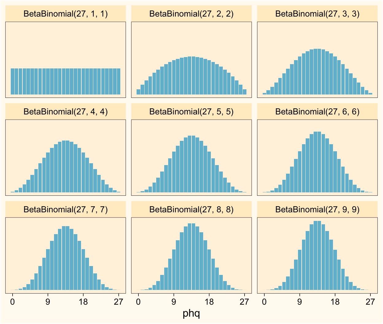
As the \(\alpha\) and \(\beta\) parameters increase, the distribution becomes more concentrated around the mean. I don’t know about you, but my experience has been that most roughly-symmetric sum-score data tend to look about like the distributions in \(\operatorname{BetaBinomial}(27, 3, 3)\) through \(\operatorname{BetaBinomial}(27, 7, 7)\).

Using the formula from above, here are the expected standard deviations from each of the 9 distributions.

tibble(n = 27,
       a = 1:9) %>% 
  mutate(b = a) %>% 
  mutate(variance = (n * a * b * (a + b + n)) / ((a + b)^2 * (a + b + 1))) %>% 
  mutate(standard_deviation = sqrt(variance))

## # A tibble: 9 × 5
##       n     a     b variance standard_deviation
##   <dbl> <int> <int>    <dbl>              <dbl>
## 1    27     1     1     65.2               8.08
## 2    27     2     2     41.8               6.47
## 3    27     3     3     31.8               5.64
## 4    27     4     4     26.2               5.12
## 5    27     5     5     22.7               4.76
## 6    27     6     6     20.2               4.5 
## 7    27     7     7     18.4               4.30
## 8    27     8     8     17.1               4.13
## 9    27     9     9     16.0               4.00

If you’re in a total state of ignorance, it’s hard to know which one’s best. But I think we’re in the right ballpark, here.

Recap.

• Popoviciu’s inequality gave us a possible range for \(\sigma\), which was between 0 and 13.5 for our PHQ-9 example.
• When we used the uniform distribution as a rough null default, the expected standard deviation was about 7.8.
• When we used plausible candidate beta-binomial distributions, we got \(\sigma\) values ranging from 6 to 4, depending on which seems like the best default.

Thus, if I were to try modeling actual PHQ-9 data for the first time, and I had no access to all the previous studies using the PHQ-9, I’d set something like

$$ \sigma \sim \operatorname{Exponential}(1 / 5.641049), $$

based of the expected standard deviation from \(\operatorname{BetaBinomial}(27, 3, 3)\). Here’s what that prior looks like:

# 1 / 5.641049 is about 0.177272
prior(exponential(0.177272)) %>% 
  parse_dist() %>% 
  ggplot(aes(y = 0, dist = .dist, args = .args)) +
  stat_halfeye(point_interval = mean_qi, .width = c(.5, .95),
               fill = h[6]) +
  scale_y_continuous(NULL, breaks = NULL) +
  labs(title = "Exponential(1 / 5.641049)",
       x = NULL)

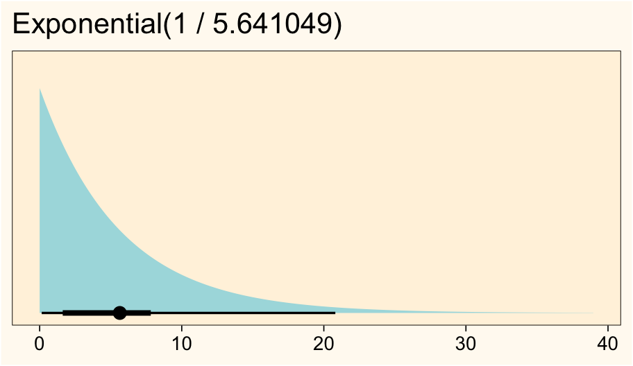
Such a distribution puts the inner 50% of the prior mass between 1.6 and 7.8, which is centered where I want it. The exponential prior, by default, holds the standard deviation constant with the mean. If you wanted a stronger prior with a smaller standard deviation, you could switch to a 2-parameter distribution like the gamma or lognormal.

# to compute the 50% and 95% ranges, execute this code
qexp(p = c(0.25, 0.75), rate = 1 / 5.641049)    # 50% interval
qexp(p = c(0.025, 0.975), rate = 1 / 5.641049)  # 95% interval

If you’re not familiar with using the exponential distribution for \(\sigma\) priors, check out the second edition of McElreath’s textbook. In chapter 4, he made the case the exponential distribution can be a good option when you have a sense of where the mean of the prior should be, but you’re unsure how large you want its spread. I’ve found it pretty handy over the past couple years.

Applied example

Okay, that’s enough theory. Let’s see how this works in practice.

We need data.

In response to a call on twitter, neuroscience graduate student Sam Zorowitz kindly shared some de-identified PHQ-9 data collected by the good folks in the Niv Lab. I’ve saved the file on GitHub. Here we’ll load the data and save them as phq9.

# load
phq9 <- read_csv("data/phq9.csv")

# what is this?
glimpse(phq9)

## Rows: 4,500
## Columns: 4
## $ subject  <dbl> 1, 1, 1, 1, 1, 1, 1, 1, 1, 2, 2, 2, 2, 2, 2, 2, 2, 2, 3, 3, 3…
## $ item     <dbl> 1, 2, 3, 4, 5, 6, 7, 8, 9, 1, 2, 3, 4, 5, 6, 7, 8, 9, 1, 2, 3…
## $ order    <dbl> 1, 6, 10, 3, 9, 8, 4, 5, 7, 3, 2, 8, 10, 4, 5, 1, 9, 6, 3, 5,…
## $ response <dbl> 1, 0, 2, 2, 0, 0, 1, 0, 0, 0, 1, 1, 2, 0, 1, 0, 0, 0, 2, 3, 3…

These data are a subset of \(n = 500\) cases, which Zorowitz randomly drew from a larger pool of \(N \approx 10{,}000\) cases. In a personal communication (11-30-2022), Zorowitz reported his team plans to make the full parent data set publicly available in the near future. In the meantime, this \(n = 500\) subset is more than enough for our purposes. In this file:

• subject: anonymized participant ID
• item: the unique item on the PHQ-9
• order: the position of the item on the webpage as presented to that participant
• response: the participant’s response

As we’d expect, the response values range from 0 to 3.

phq9 %>% 
  count(response)

## # A tibble: 4 × 2
##   response     n
##      <dbl> <int>
## 1        0  1939
## 2        1  1392
## 3        2   726
## 4        3   443

Happily, there are no missing values to contend with. Since our focus is on the sum scores, rather than the items, we’ll need to wrangle the data a bit.

phq9 <- phq9 %>% 
  group_by(subject) %>% 
  summarise(phq = sum(response)) %>% 
  ungroup()

# what?
glimpse(phq9)

## Rows: 500
## Columns: 2
## $ subject <dbl> 1, 2, 3, 4, 5, 6, 7, 8, 9, 10, 11, 12, 13, 14, 15, 16, 17, 18,…
## $ phq     <dbl> 6, 5, 16, 3, 8, 9, 13, 13, 7, 4, 2, 4, 3, 13, 3, 7, 8, 0, 10, …

Now the sum scores are in the phq column. Though we don’t technically need to, it will help me make my point if we subset the data further to \(n = 200\). We can take a random subset with the slice_sample() function.

set.seed(9)

phq9 <- phq9 %>% 
  slice_sample(n = 200)

# confirm the sample size
nrow(phq9)

## [1] 200

Here’s what the data look like.

phq9 %>% 
  ggplot(aes(x = phq)) +
  geom_bar(fill = h[3]) +
  scale_x_continuous(breaks = 0:3 * 9, limits = c(-0.5, 27.5))

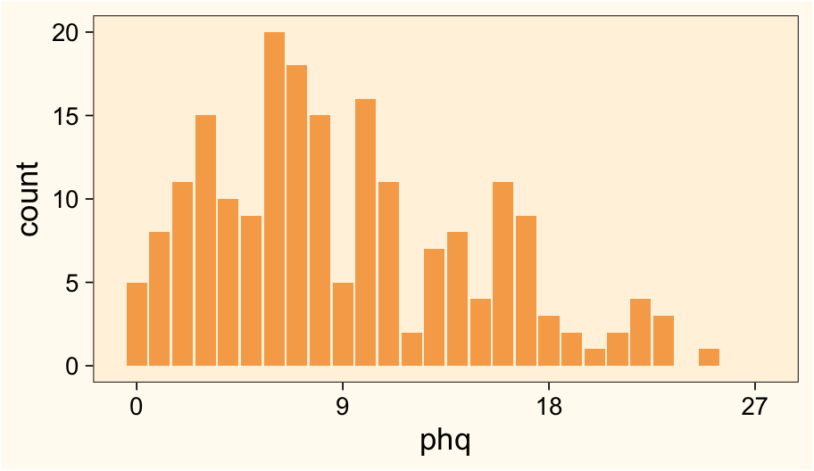
Based on my experience, this is a pretty typical distribution for the PHQ-9.

We need a model.

For the sake of the blog, let’s keep things simple and fit an intercept-only model of the phq scores. In the real world, I actually know a lot about the PHQ-9 and there’s a mountain of prior studies reporting sample statistics for its sum score. But if this weren’t the case and we were trying to fit a model in a state of near-complete ignorance, I think a pretty great place to start would be

$$ \begin{align*} \text{PHQ-9}_i & \sim \operatorname{Normal}(\mu, \sigma) \\ \mu & = \beta_0 \\ \beta_0 & \sim \operatorname{Normal}(13.5, 5.641049) \\ \sigma & \sim \operatorname{Exponential}(1 / 5.641049), \end{align*} $$

where the top line indicates the PHQ-9 scores vary across the \(i\) cases, and the scores are described as following the normal distribution. The second line of the equation indicates this is an intercept-only model, with \(\beta_0\) defining the intercept. Skipping the third line for a moment, the fourth line shows we’ve chosen an exponential prior for \(\sigma\) for which the rate is \(1 / 5.641049\) and thus the mean is \(5.641049\)⁶. Where did that value come from, again? After exploring some nice candidate beta-binomial distributions, we said \(\operatorname{BetaBinomial}(27, 3, 3)\) might be a good default option, and the expected standard deviation for that distribution is 5.641049. Here those are, again:

# define
n <- 27
a <- 3
b <- a

tibble(phq = 0:27,
       a   = a,
       b   = b) %>% 
  mutate(d = VGAM::dbetabinom.ab(x = phq, size = n, shape1 = a, shape2 = b)) %>%

  # plot
  ggplot(aes(x = phq, y = d)) +
  geom_col(fill = h[7]) +
  scale_x_continuous(breaks = 0:3 * 9) +
  scale_y_continuous(NULL, breaks = NULL) +
  ggtitle("BetaBinomial(27, 3, 3)")

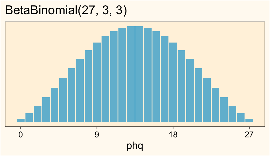
# compute the population sd
sqrt(((n * a * b) * (a + b + n)) / ((a + b)^2 * (a + b + 1)))

## [1] 5.641049

Now back to the third line in the model equation. As per usual, we have used a Gaussian prior for \(\beta_0\). We’ve centered the prior on the middle of the possible range of the sum score, which is 13.5. Since we’ve decided 5.641049 is a pretty good value for \(\sigma\), it’s not a bad idea to use that value for the scale of our \(\beta_0\) prior. Such a prior would have an inner 95% range of about 2.4 to 22.6, which covers most of the possible sum-score range.

qnorm(p = c(0.025, 0.975), mean = 13.5, sd = 5.641049)

## [1]  2.443747 24.556253

Otherwise put, the full range of the PHQ-9 sum score is 13.5 plus or minus 2.4 standard deviations, as defined by our \(\sigma\) prior.

13.5 / 5.641049

## [1] 2.393172

F* around and find out.⁷

Here’s how to fit the model with brm().

fit1 <- brm(
  data = phq9,
  family = gaussian,
  phq ~ 1,
  prior(normal(13.5, 5.641049), class = Intercept) +
    prior(exponential(1 / 5.641049), class = sigma),
  cores = 4, seed = 1
)

Check the model summary.

summary(fit1)

##  Family: gaussian 
##   Links: mu = identity; sigma = identity 
## Formula: phq ~ 1 
##    Data: phq9 (Number of observations: 200) 
##   Draws: 4 chains, each with iter = 2000; warmup = 1000; thin = 1;
##          total post-warmup draws = 4000
## 
## Population-Level Effects: 
##           Estimate Est.Error l-95% CI u-95% CI Rhat Bulk_ESS Tail_ESS
## Intercept     9.04      0.41     8.24     9.83 1.00     3009     2271
## 
## Family Specific Parameters: 
##       Estimate Est.Error l-95% CI u-95% CI Rhat Bulk_ESS Tail_ESS
## sigma     5.81      0.29     5.27     6.43 1.00     3468     2246
## 
## Draws were sampled using sampling(NUTS). For each parameter, Bulk_ESS
## and Tail_ESS are effective sample size measures, and Rhat is the potential
## scale reduction factor on split chains (at convergence, Rhat = 1).

At a glance, everything looks fine. It might be more instructive to look the results in a couple plots where we compare the priors with the posteriors.

# intercept
p1 <- as_draws_df(fit1) %>% 
  ggplot(aes(x = b_Intercept, y = after_stat(density))) +
  geom_area(data = tibble(b_Intercept = seq(-5, 30, by = 0.01),
                          density = dnorm(b_Intercept, 13.5, 5.641049)),
            aes(y = density),
            fill = h[10]) +
  geom_histogram(fill = alpha(h[2], 2/3), boundary = 0, binwidth = 0.2) +
  scale_x_continuous(expression(beta[0]), breaks = 0:3 * 9) +
  scale_y_continuous(NULL, breaks = NULL) +
  coord_cartesian(xlim = c(0, 27))

# sigma
p2 <- as_draws_df(fit1) %>% 
  ggplot(aes(x = sigma, y = after_stat(density))) +
  geom_area(data = tibble(sigma = seq(0, 20, by = 0.01),
                          density = dexp(sigma, 1 / 5.641049)),
            aes(y = density),
            fill = h[10]) +
  geom_histogram(fill = alpha(h[2], 2/3), boundary = 0, binwidth = 0.1) +
  geom_vline(xintercept = 13.5, linetype = 2, color = h[1]) +
  annotate(geom = "text",
           x = 13.3, y = 1.37,
           label = "Upper limit via\nPopoviciu's inequality",
           hjust = 1, size = 3) +
  scale_x_continuous(expression(sigma), breaks = 0:3 * 5) +
  scale_y_continuous(NULL, breaks = NULL) +
  coord_cartesian(xlim = c(0, 15))

# combine
(p1 | p2) &
  plot_annotation(title = "Careful priors can express our substantive ignorance, but still\naccount for our methodological knowledge.",
                  subtitle = "The prior densities lurk in the background. The posteriors are the\nsemitransparent orange histograms in the foreground.")

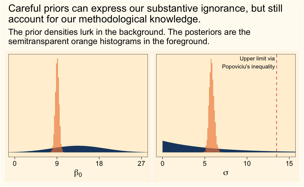
It looks like both priors did their jobs well.

Objections

But the data were skewed!

Some readers might not like how we centered the prior for \(\beta_0\) or how we used a symmetric beta-binomial distribution to determine the prior for \(\sigma\) given how the actual PHQ-9 data were skewed to the right, and given how PHQ-9 data are very often skewed to the right in other samples. Keep in mind that our focus is a strategy which will work when we don’t have information like that going in. When you’re completely ignorant of how your sum-score data tend to look, I recommend assuming they’ll be roughly symmetric.

However, it’s possible some of y’all work in fields where your sum-scores are routinely skewed in one direction or the other. If so, great! That means you have useful domain knowledge upon which you can base your priors. One of the nice things about the beta-binomial distribution is it can take on a variety of non-symmetric shapes. For example, take a look at the distribution of \(\operatorname{BetaBinomial}(27, 1.5, 3.25)\).

# define
n <- 27
a <- 1.5
b <- 3.25

tibble(phq = 0:27,
       a   = a,
       b   = b) %>% 
  mutate(d = VGAM::dbetabinom.ab(x = phq, size = n, shape1 = a, shape2 = b)) %>% 

  # plot
  ggplot(aes(x = phq, y = d)) +
  geom_col(fill = h[7]) +
  scale_x_continuous(breaks = 0:3 * 9) +
  scale_y_continuous(NULL, breaks = NULL) +
  ggtitle("BetaBinomial(27, 1.5, 3.25)")

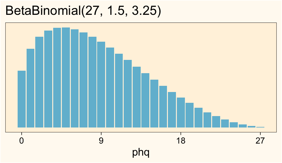
This looks a lot like the empirical distribution in our phq9 data, doesn’t it? We could then use this skewed version of the beta-binomial to compute the expected standard deviation.

# compute the population sd
sqrt(((n * a * b) * (a + b + n)) / ((a + b)^2 * (a + b + 1)))

## [1] 5.675623

So if you were working with questionnaire data in a domain where you expected the sum-score to have this kind of skewed distribution, you might assume \(\sigma \sim \operatorname{Exponential}(1 / 5.675623)\). It’s worth spending some time plotting beta-binomial distributions with different values for its \(n\), \(\alpha\), and \(\beta\) parameters. Scientists working in different research domains might prefer different default versions of the distribution.

Just standardize.

If you wanted to take a different approach, you could just standardize the sum-score data before the analysis and then fit the model to the standardized values. This is a fine practice and it would greatly simplify how you choose your priors. I do this on occasion, myself. However, sometimes I want to fit the model to the un-transformed data and I’d like a workflow that can work on those occasions. This is such a workflow.

Plus, like, do you really care so little about your data and your research questions that you don’t want to put a little thought into what you expect the data will look like? If not, maybe science isn’t a good fit for you.⁸

You sure about that Gauss?

Some readers might wonder whether it’s such a great idea to model sum-score data with the conventional Gaussian likelihood. The Gauss expects truly continuous data, and it doesn’t have a natural way to handle data with well-defined minimum and maximum values. The Gaussian likelihood might not be the best when dealing with markedly-skewed data, either.

One alternative would be using skew-normal or skew-Student likelihood. For details, see the ( 2017) preprint by Martin and Williams. This approach, however, will not fully solve the problem with the lower and upper boundaries. A more sophisticated approach would be to model the item-level data with a multilevel-ordinal IRT-type model, such as discussed by Bürkner ( 2020). This approach is excellent for respecting the ordinal nature of the questionnaire items and for expressing the data-generating process, but it comes at the cost of a complex, highly-parameterized model which may be difficult to fit and explain in a manuscript.

If you’ve been following along, another option is to model the sum scores as beta-binomial. This approach would account for skew, upper and lower boundaries, and for the integer values. The beta-binomial would not faithfully reproduce the item-level data-generating process, but you might think of it as a pragmatic and simpler alternative to the rigorous item-level multilevel-ordinal IRT approach. This approach is possible with brm() by setting family = beta_binomial. Though it’s beyond the scope of this blog post, I’ve been chipping away at a blog series which will explore the beta-binomial distribution for sum-score data. As a preview, here’s how to fit such a model to these data.

fit2 <- brm(
  data = phq9,
  family = beta_binomial,
  phq | trials(27) ~ 1,
  prior(normal(0, 1), class = Intercept) +
    prior(gamma(2.25, 0.375), class = phi),
  cores = 4, seed = 1
)

Whichever method you use in your research, I hope this post gave you some helpful ideas. Happy modeling, friends!

Session info

sessionInfo()

## R version 4.2.0 (2022-04-22)
## Platform: x86_64-apple-darwin17.0 (64-bit)
## Running under: macOS Big Sur/Monterey 10.16
## 
## Matrix products: default
## BLAS:   /Library/Frameworks/R.framework/Versions/4.2/Resources/lib/libRblas.0.dylib
## LAPACK: /Library/Frameworks/R.framework/Versions/4.2/Resources/lib/libRlapack.dylib
## 
## locale:
## [1] en_US.UTF-8/en_US.UTF-8/en_US.UTF-8/C/en_US.UTF-8/en_US.UTF-8
## 
## attached base packages:
## [1] stats     graphics  grDevices utils     datasets  methods   base     
## 
## other attached packages:
##  [1] MetBrewer_0.2.0 brms_2.18.0     Rcpp_1.0.9      patchwork_1.1.2
##  [5] tidybayes_3.0.2 forcats_0.5.1   stringr_1.4.1   dplyr_1.0.10   
##  [9] purrr_0.3.4     readr_2.1.2     tidyr_1.2.1     tibble_3.1.8   
## [13] ggplot2_3.4.0   tidyverse_1.3.2
## 
## loaded via a namespace (and not attached):
##   [1] readxl_1.4.1         backports_1.4.1      VGAM_1.1-7          
##   [4] plyr_1.8.7           igraph_1.3.4         svUnit_1.0.6        
##   [7] splines_4.2.0        crosstalk_1.2.0      TH.data_1.1-1       
##  [10] rstantools_2.2.0     inline_0.3.19        digest_0.6.30       
##  [13] htmltools_0.5.3      fansi_1.0.3          magrittr_2.0.3      
##  [16] checkmate_2.1.0      googlesheets4_1.0.1  tzdb_0.3.0          
##  [19] modelr_0.1.8         RcppParallel_5.1.5   matrixStats_0.62.0  
##  [22] vroom_1.5.7          xts_0.12.1           sandwich_3.0-2      
##  [25] prettyunits_1.1.1    colorspace_2.0-3     rvest_1.0.2         
##  [28] ggdist_3.2.0         haven_2.5.1          xfun_0.35           
##  [31] callr_3.7.3          crayon_1.5.2         jsonlite_1.8.3      
##  [34] lme4_1.1-31          survival_3.4-0       zoo_1.8-10          
##  [37] glue_1.6.2           gtable_0.3.1         gargle_1.2.0        
##  [40] emmeans_1.8.0        distributional_0.3.1 pkgbuild_1.3.1      
##  [43] rstan_2.21.7         abind_1.4-5          scales_1.2.1        
##  [46] mvtnorm_1.1-3        DBI_1.1.3            miniUI_0.1.1.1      
##  [49] xtable_1.8-4         bit_4.0.4            stats4_4.2.0        
##  [52] StanHeaders_2.21.0-7 DT_0.24              htmlwidgets_1.5.4   
##  [55] httr_1.4.4           threejs_0.3.3        arrayhelpers_1.1-0  
##  [58] posterior_1.3.1      ellipsis_0.3.2       pkgconfig_2.0.3     
##  [61] loo_2.5.1            farver_2.1.1         sass_0.4.2          
##  [64] dbplyr_2.2.1         utf8_1.2.2           labeling_0.4.2      
##  [67] tidyselect_1.1.2     rlang_1.0.6          reshape2_1.4.4      
##  [70] later_1.3.0          munsell_0.5.0        cellranger_1.1.0    
##  [73] tools_4.2.0          cachem_1.0.6         cli_3.4.1           
##  [76] generics_0.1.3       broom_1.0.1          ggridges_0.5.3      
##  [79] evaluate_0.18        fastmap_1.1.0        yaml_2.3.5          
##  [82] bit64_4.0.5          processx_3.8.0       knitr_1.40          
##  [85] fs_1.5.2             nlme_3.1-159         mime_0.12           
##  [88] projpred_2.2.1       xml2_1.3.3           compiler_4.2.0      
##  [91] bayesplot_1.9.0      shinythemes_1.2.0    rstudioapi_0.13     
##  [94] gamm4_0.2-6          reprex_2.0.2         bslib_0.4.0         
##  [97] stringi_1.7.8        highr_0.9            ps_1.7.2            
## [100] blogdown_1.15        Brobdingnag_1.2-8    lattice_0.20-45     
## [103] Matrix_1.4-1         nloptr_2.0.3         markdown_1.1        
## [106] shinyjs_2.1.0        tensorA_0.36.2       vctrs_0.5.0         
## [109] pillar_1.8.1         lifecycle_1.0.3      jquerylib_0.1.4     
## [112] bridgesampling_1.1-2 estimability_1.4.1   httpuv_1.6.5        
## [115] R6_2.5.1             bookdown_0.28        promises_1.2.0.1    
## [118] gridExtra_2.3        codetools_0.2-18     boot_1.3-28         
## [121] colourpicker_1.1.1   MASS_7.3-58.1        gtools_3.9.3        
## [124] assertthat_0.2.1     withr_2.5.0          shinystan_2.6.0     
## [127] multcomp_1.4-20      mgcv_1.8-40          parallel_4.2.0      
## [130] hms_1.1.1            grid_4.2.0           coda_0.19-4         
## [133] minqa_1.2.5          rmarkdown_2.16       googledrive_2.0.0   
## [136] numDeriv_2016.8-1.1  shiny_1.7.2          lubridate_1.8.0     
## [139] base64enc_0.1-3      dygraphs_1.1.1.6

References

Bürkner, P.-C. (2020). Bayesian item response modeling in R with brms and Stan. http://arxiv.org/abs/1905.09501
Bürkner, P.-C. (2017). brms: An R package for Bayesian multilevel models using Stan. Journal of Statistical Software, 80(1), 1–28. https://doi.org/10.18637/jss.v080.i01
Bürkner, P.-C. (2018). Advanced Bayesian multilevel modeling with the R package brms. The R Journal, 10(1), 395–411. https://doi.org/10.32614/RJ-2018-017
Bürkner, P.-C. (2022). brms: Bayesian regression models using ’Stan’. https://CRAN.R-project.org/package=brms
Carlin, J. B., & Rubin, D. B. (1991). Summarizing multiple-choice tests using three informative statistics. Psychological Bulletin, 110(2), 338–349. https://doi.org/10.1037/0033-2909.110.2.338
Gelman, A., Hill, J., & Vehtari, A. (2020). Regression and other stories. Cambridge University Press. https://doi.org/10.1017/9781139161879
Greenleaf, E. A. (1992). Measuring extreme response style. Public Opinion Quarterly, 56(3), 328–351. https://doi.org/10.1086/269326
Kay, M. (2022). tidybayes: Tidy data and ’geoms’ for Bayesian models. https://CRAN.R-project.org/package=tidybayes
Kruschke, J. K. (2015). Doing Bayesian data analysis: A tutorial with R, JAGS, and Stan. Academic Press. https://sites.google.com/site/doingbayesiandataanalysis/
Lord, F. M. (1962). Estimating true measurements from fallible measurements (binomial case)expansion in a series of beta distributions. ETS Research Bulletin Series, 1962(2), i–26. https://doi.org/10.1002/j.2333-8504.1962.tb00301.x
Martin, S. R., & Williams, D. R. (2017). Outgrowing the Procrustean bed of normality: The utility of Bayesian modeling for asymmetrical data analysis. https://doi.org/10.31234/osf.io/26m49
McElreath, R. (2020). Statistical rethinking: A Bayesian course with examples in R and Stan (Second Edition). CRC Press. https://xcelab.net/rm/statistical-rethinking/
McElreath, R. (2015). Statistical rethinking: A Bayesian course with examples in R and Stan. CRC press. https://xcelab.net/rm/statistical-rethinking/
Mills, B. R. (2022). MetBrewer: Color palettes inspired by works at the Metropolitan Museum of Art. https://CRAN.R-project.org/package=MetBrewer
Pedersen, T. L. (2022). patchwork: The composer of plots. https://CRAN.R-project.org/package=patchwork
Popoviciu, T. (1935). Sur les équations algébriques ayant toutes leurs racines réelles. Mathematica Cluj, 9(129-145).
Spitzer, R. L., Kroenke, K., Williams, J. B., Group, P. H. Q. P. C. S., Group, P. H. Q. P. C. S., et al. (1999). Validation and utility of a self-report version of PRIME-MD: The PHQ primary care study. JAMA, 282(18), 1737–1744. https://doi.org/10.1001/jama.282.18.1737
Wickham, H. (2022). tidyverse: Easily install and load the ’tidyverse’. https://CRAN.R-project.org/package=tidyverse
Wickham, H., Averick, M., Bryan, J., Chang, W., McGowan, L. D., François, R., Grolemund, G., Hayes, A., Henry, L., Hester, J., Kuhn, M., Pedersen, T. L., Miller, E., Bache, S. M., Müller, K., Ooms, J., Robinson, D., Seidel, D. P., Spinu, V., … Yutani, H. (2019). Welcome to the tidyverse. Journal of Open Source Software, 4(43), 1686. https://doi.org/10.21105/joss.01686
Wilcox, R. R. (1981). A review of the beta-binomial model and its extensions. Journal of Educational Statistics, 6(1), 3–32. https://doi.org/10.2307/1165046
Yee, T. (2022). VGAM: Vector generalized linear and additive models. https://www.stat.auckland.ac.nz/~yee/VGAM/
-
Or if you’re thinking in terms of OLS, presume the residuals are normally distributed. ↩︎
We use the PHQ-9 all the time in the VA (i.e., the US Department of Veterans Affairs) both in clinical services and in research settings. It’s reasonably brief and it does a fair job assessing the primary diagnostic criteria for major depressive disorder. ↩︎
If you increase the
nof the sample, you’ll see the sample statistics quickly approach the values from Popoviciu’s inequality. ↩︎ -
There’s the whole ‘Fisher liked the normal distribution, so you should too’ bit. Plus we do need defaults and the Gaussian isn’t a bad candidate, all things considered. But yeah, sigh ↩︎
Yes, I know; some is doing a lot of work, here. ↩︎
If you didn’t know, the rate of the exponential distribution is the reciprocal of its mean. ↩︎
In case you’re not in on the joke, behold: https://youtu.be/d6sbPCIEMyI ↩︎
Okay, I admit that was a little snarky. But what are we really doing here? Are we just churning out
\(p\)-values for pubs or does the science matter at all? ↩︎