Yes, you can compute standardized regression coefficients with multiple imputation

What?

All the players know there are three major ways to handle missing data:

• full-information maximum likelihood,
• multiple imputation, and
• one-step full-luxury¹ Bayesian imputation.

In an earlier post, we walked through method for plotting the fitted lines from models fit with multiply-imputed data. In this post, we’ll discuss another neglected topic: How might one compute standardized regression coefficients from models fit with multiply-imputed data?

I make assumptions.

For this post, I’m presuming some background knowledge:

• You should be familiar with regression. For frequentist introductions, I recommend Roback and Legler’s ( 2021) online text or James, Witten, Hastie, and Tibshirani’s ( 2021) online text. For Bayesian introductions, I recommend either edition of McElreath’s text ( 2015, 2020); Kruschke’s ( 2015) text; or Gelman, Hill, and Vehtari’s ( 2020) text.

• You should be familiar with contemporary missing data theory. You can find brief overviews in the texts by McElreath and Gelman et al, above. For a deeper dive, I recommend Enders ( 2022), Little & Rubin ( 2019), or van Buuren ( 2018).

• All code is in R. Data wrangling and plotting were done with help from the tidyverse ( Wickham et al., 2019; Wickham, 2022) and ggside ( Landis, 2022). The data and multiple-imputation workflow are from the mice package ( van Buuren & Groothuis-Oudshoorn, 2011, 2021).

Here we load our primary R packages.

library(tidyverse)
library(ggside)
library(mice)

We need data.

In this post we’ll use the nhanes data set ( Schafer, 1997).

data(nhanes, package = "mice")

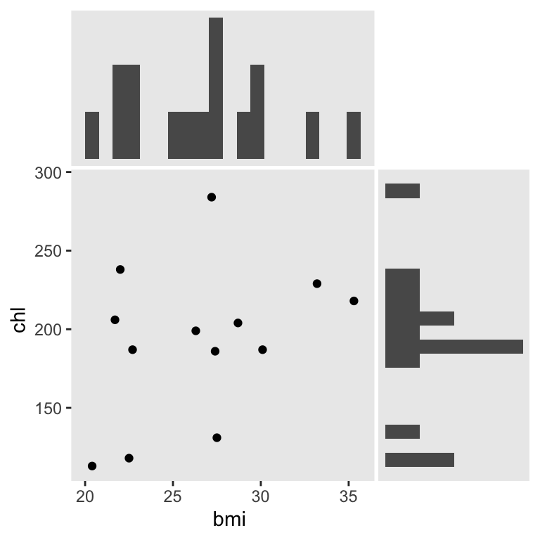
We’ll be focusing on the two variables, bmi and chl. Here’s a look at their univarite and bivariate distributions.

nhanes %>% 
  ggplot(aes(x = bmi, y = chl)) +
  geom_point() +
  geom_xsidehistogram(bins = 20) +
  geom_ysidehistogram(bins = 20) +
  scale_xsidey_continuous(breaks = NULL) +
  scale_ysidex_continuous(breaks = NULL) +
  theme(axis.title = element_text(hjust = 1/3),
        ggside.panel.scale = 0.5,
        panel.grid = element_blank())

We can use mice::md.pattern() to reveal their four distinct missing data patterns.

nhanes %>% 
  select(bmi, chl) %>% 
  md.pattern()

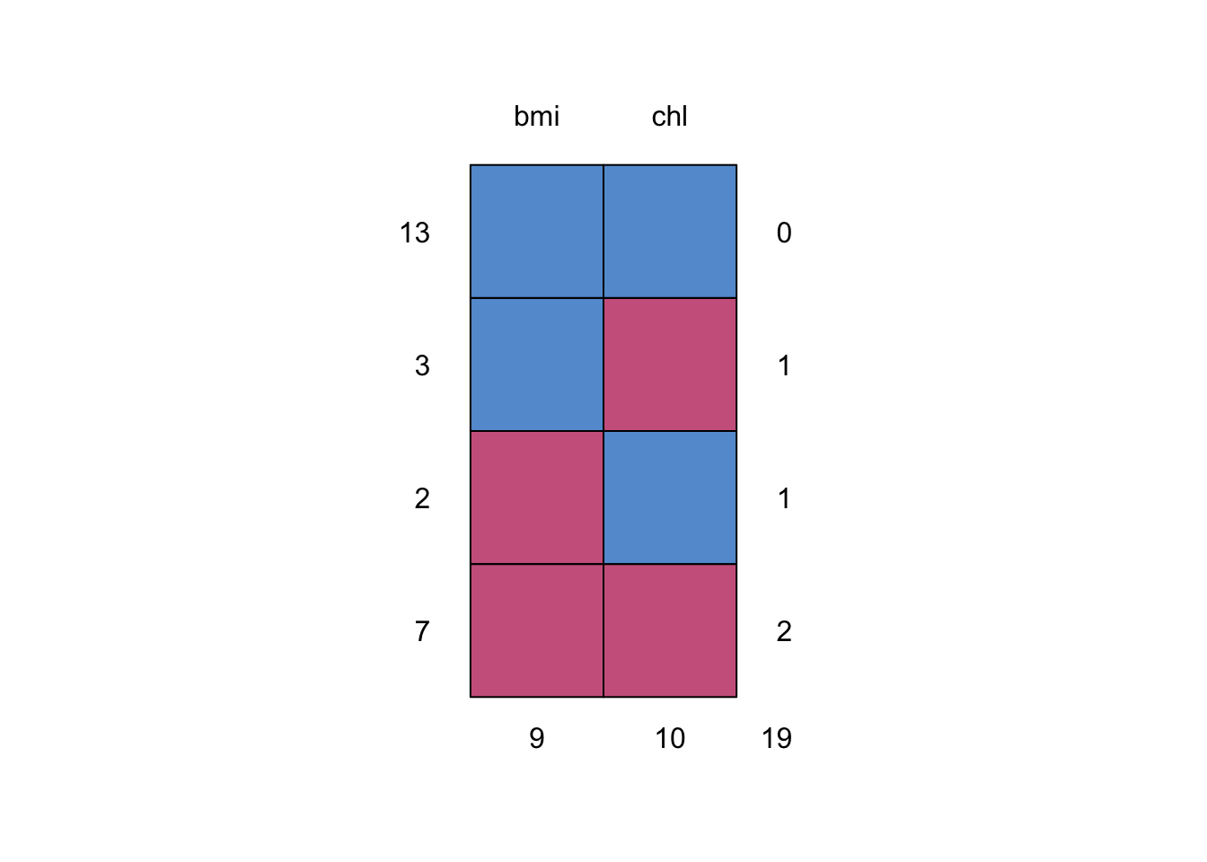
##    bmi chl   
## 13   1   1  0
## 3    1   0  1
## 2    0   1  1
## 7    0   0  2
##      9  10 19

We’re missing nine cases in bmi and missing 10 cases in chl.

Impute

We’ll use the mice() function to impute. By setting m = 100, we’ll get back 100 multiply-imputed data sets. By setting method = "norm", we will be using Bayesian linear regression with the Gaussian likelihood to compute the imputed values. The seed argument makes our results reproducible.

imp <- nhanes %>% 
  select(bmi, chl) %>% 
  mice(seed = 1, m = 100, method = "norm", print = FALSE)

Model

Our basic model will be

$$ \begin{align*} \text{chl}_i & \sim \operatorname{Gaussian}(\mu_i, \sigma) \\ \mu_i & = \beta_0 + \beta_1 \text{bmi}_i, \end{align*} $$

where bmi is the sole predictor of chl. Here’s how we use the with() function to fit that model to each of the 100 imputed data sets.

fit1 <- with(imp, lm(chl ~ 1 + bmi))

We use the pool() function to pool the results from the 100 MI data sets according to Rubin’s rules ( Little & Rubin, 2019; Rubin, 1987).

pooled1 <- pool(fit1)

Now we can summarize the results.

summary(pooled1, conf.int = T)

##          term  estimate std.error statistic       df   p.value      2.5 %
## 1 (Intercept) 97.798132 74.951754  1.304814 12.36661 0.2157149 -64.972384
## 2         bmi  3.558074  2.765967  1.286376 12.63050 0.2213919  -2.435254
##       97.5 %
## 1 260.568649
## 2   9.551402

Since I’m not an expert in the nhanes data, it’s hard to know how impressed I should be with the 3.6 estimate for bmi. An effect size could help.

Standadrdized coefficients with van Ginkel’s proposal

In his ( 2020) paper, Standardized regression coefficients and newly proposed estimators for \(R^2\) in multiply imputed data, Joost van Ginkel presented two methods for computing standardized regression coefficients from multiply imputed data. van Ginkel called these two methods \(\bar{\hat\beta}_\text{PS}\), which stands for Pooling before Standardization, and \(\bar{\hat\beta}_\text{SP}\), which stands for Standardization before Pooling. In the paper, he showed both methods are pretty good in terms of bias and coverage. I find the SP approach intuitive and easy to use, so that’s the one we’ll be using in this post.

For the SP method, we don’t need to change our mice()-based imputation step from above. The big change is how we fit the model with lm() and with(). As van Ginkel covered in the paper, one of the ways you might compute standardized regression coefficients is by fitting the model with standardized variables. Instead of messing with the actual imp data, we can simply standardize the variables directly in the model formula within lm() by way of the base-R scale() function.

fit2 <- with(imp, lm(scale(chl) ~ 1 + scale(bmi)))

I should note it was Mattan S. Ben-Shachar who came up with the scale() insight for our with() implementation.

with(mids, lm(scale(y) ~ scale(x) + scale(z)))

— Mattan S. Ben-Shachar ❤️‍🩹🎗️ (@mattansb) October 7, 2022

While I’m at it, it was Isabella R. Ghement who directed me to the van Ginkel paper.

Solomon, did you see this article - it seems to discuss what you need:

“Standardized Regression Coefficients and Newly Proposed Estimators for in Multiply Imputed Data”
Joost R. van Ginkelhttps://t.co/auSvA68IR9

— Isabella R. Ghement (@IsabellaGhement) October 8, 2022

Anyway, now we’ve fit the standardized model, we can pool as normal.

pooled2 <- pool(fit2)

Here are the results.

summary(pooled2, conf.int = T)

##          term      estimate std.error     statistic       df   p.value
## 1 (Intercept) -1.838514e-17 0.1905258 -9.649687e-17 21.22865 1.0000000
## 2  scale(bmi)  3.275347e-01 0.2476081  1.322795e+00 12.84446 0.2089718
##        2.5 %    97.5 %
## 1 -0.3959603 0.3959603
## 2 -0.2080493 0.8631187

The standardized regression coefficient for bmi is \(0.33\), \(95\% \text{CI}\) \([-0.21, 0.86]\). As we only have one predictor, the standardized coefficient is in a correlation metric, which makes it easy to interpret the point estimate.

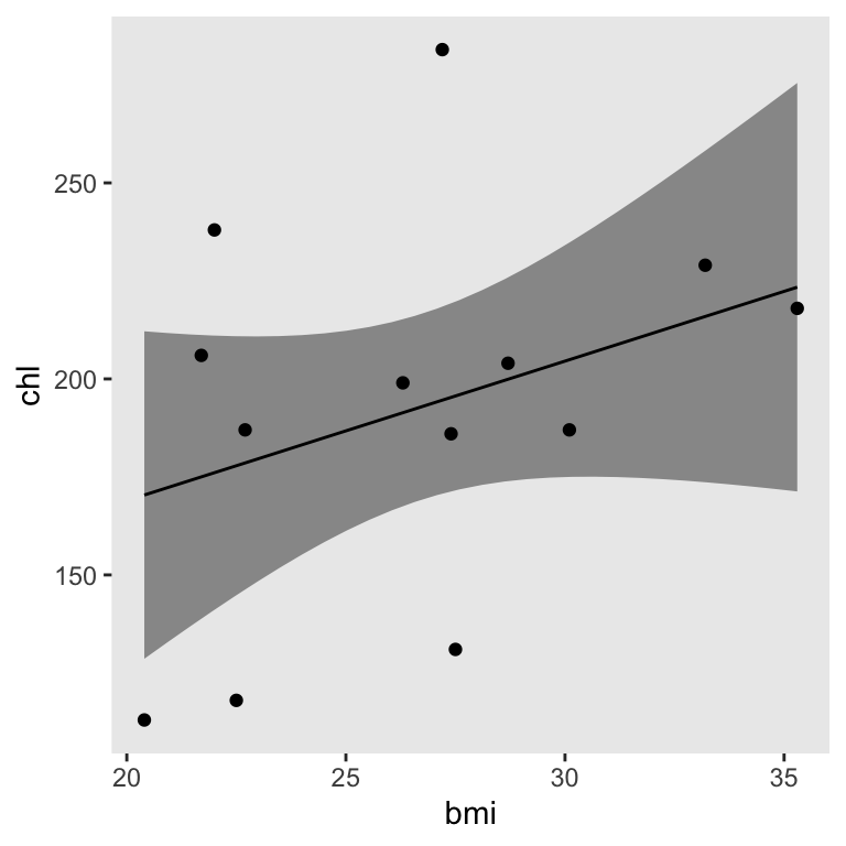
Just for kicks, here’s how you might plot the pooled fitted line and its pooled 95% interval using the method from an earlier post.

# define the total number of imputations
m <- 100

# define the new data
nd <- tibble(bmi = seq(from = min(nhanes$bmi, na.rm = T), to = max(nhanes$bmi, na.rm = T), length.out = 30))

# compute the fitted values, by imputation
tibble(.imp = 1:100) %>% 
  mutate(p = map(.imp, ~ predict(fit1$analyses[[.]], 
                                 newdata = nd, 
                                 se.fit = TRUE) %>% 
                   data.frame())
         ) %>% 
  unnest(p) %>%
  # add in the nd predictor data
  bind_cols(
    bind_rows(replicate(100, nd, simplify = FALSE))
    ) %>% 
  # drop two unneeded columns
  select(-df, -residual.scale) %>% 
  group_by(bmi) %>% 
  # compute the pooled fitted values and the pooled standard errors
  summarise(fit_bar = mean(fit),
            v_w     = mean(se.fit^2),
            v_b     = sum((fit - fit_bar)^2) / (m - 1),
            v_p     = v_w + v_b * (1 + (1 / m)),
            se_p    = sqrt(v_p)) %>% 
  # compute the pooled 95% intervals
  mutate(lwr_p = fit_bar - se_p * 1.96,
         upr_p = fit_bar + se_p * 1.96) %>%
  
  # plot!
  ggplot(aes(x = bmi)) +
  geom_ribbon(aes(ymin = lwr_p, ymax = upr_p),
              alpha = 1/2) +
  geom_line(aes(y = fit_bar), 
            linewidth = 1/2) +
  geom_point(data = nhanes,
             aes(y = chl)) +
  labs(y = "chl") +
  theme(panel.grid = element_blank())

Limitation

To my knowledge, van Ginkel ( 2020) is the first and only methodological paper to discuss standardized regression coefficients with multiply imputed data. In the abstract, for example, van Ginkel reported: “No combination rules for standardized regression coefficients and their confidence intervals seem to have been developed at all.” Though this initial method has its strengths, it has one major limitation: The \(t\)-tests will tend to differ between the standardized and unstandardized models. To give a sense, let’s compare the results from our unstandardized and standardized models.

# unstandardized t-test
summary(pooled1, conf.int = T)[2, "statistic"]

## [1] 1.286376

# standardized t-test
summary(pooled2, conf.int = T)[2, "statistic"]

## [1] 1.322795

Yep, they’re a little different. van Ginkel covered this issue in his Discussion section, the details of which I’ll leave to the interested reader. This limitation notwithstanding, van Ginkel ultimately preferred the SP method. 🤷 We can’t have it all, friends.

Happy modeling!

Session info

sessionInfo()

## R version 4.3.0 (2023-04-21)
## Platform: aarch64-apple-darwin20 (64-bit)
## Running under: macOS Ventura 13.4
## 
## Matrix products: default
## BLAS:   /Library/Frameworks/R.framework/Versions/4.3-arm64/Resources/lib/libRblas.0.dylib 
## LAPACK: /Library/Frameworks/R.framework/Versions/4.3-arm64/Resources/lib/libRlapack.dylib;  LAPACK version 3.11.0
## 
## locale:
## [1] en_US.UTF-8/en_US.UTF-8/en_US.UTF-8/C/en_US.UTF-8/en_US.UTF-8
## 
## time zone: America/Chicago
## tzcode source: internal
## 
## attached base packages:
## [1] stats     graphics  grDevices utils     datasets  methods   base     
## 
## other attached packages:
##  [1] mice_3.16.0     ggside_0.2.2    lubridate_1.9.2 forcats_1.0.0  
##  [5] stringr_1.5.0   dplyr_1.1.2     purrr_1.0.1     readr_2.1.4    
##  [9] tidyr_1.3.0     tibble_3.2.1    ggplot2_3.4.2   tidyverse_2.0.0
## 
## loaded via a namespace (and not attached):
##  [1] gtable_0.3.3     shape_1.4.6      xfun_0.39        bslib_0.5.0     
##  [5] lattice_0.21-8   tzdb_0.4.0       vctrs_0.6.3      tools_4.3.0     
##  [9] generics_0.1.3   fansi_1.0.4      highr_0.10       pan_1.6         
## [13] pkgconfig_2.0.3  jomo_2.7-6       Matrix_1.5-4     assertthat_0.2.1
## [17] lifecycle_1.0.3  farver_2.1.1     compiler_4.3.0   munsell_0.5.0   
## [21] codetools_0.2-19 htmltools_0.5.5  sass_0.4.6       yaml_2.3.7      
## [25] glmnet_4.1-7     crayon_1.5.2     nloptr_2.0.3     pillar_1.9.0    
## [29] jquerylib_0.1.4  MASS_7.3-58.4    cachem_1.0.8     iterators_1.0.14
## [33] rpart_4.1.19     boot_1.3-28.1    foreach_1.5.2    mitml_0.4-5     
## [37] nlme_3.1-162     tidyselect_1.2.0 digest_0.6.31    stringi_1.7.12  
## [41] bookdown_0.34    labeling_0.4.2   splines_4.3.0    fastmap_1.1.1   
## [45] grid_4.3.0       colorspace_2.1-0 cli_3.6.1        magrittr_2.0.3  
## [49] emo_0.0.0.9000   survival_3.5-5   utf8_1.2.3       broom_1.0.5     
## [53] withr_2.5.0      scales_1.2.1     backports_1.4.1  timechange_0.2.0
## [57] rmarkdown_2.22   nnet_7.3-18      lme4_1.1-33      blogdown_1.17   
## [61] hms_1.1.3        evaluate_0.21    knitr_1.43       rlang_1.1.1     
## [65] Rcpp_1.0.10      glue_1.6.2       rstudioapi_0.14  minqa_1.2.5     
## [69] jsonlite_1.8.5   R6_2.5.1

References

Enders, C. K. (2022). Applied missing data analysis (Second Edition). Guilford Press. http://www.appliedmissingdata.com/
Gelman, A., Hill, J., & Vehtari, A. (2020). Regression and other stories. Cambridge University Press. https://doi.org/10.1017/9781139161879
James, G., Witten, D., Hastie, T., & Tibshirani, R. (2021). An introduction to statistical learning with applications in R (Second Edition). Springer. https://web.stanford.edu/~hastie/ISLRv2_website.pdf
Kruschke, J. K. (2015). Doing Bayesian data analysis: A tutorial with R, JAGS, and Stan. Academic Press. https://sites.google.com/site/doingbayesiandataanalysis/
Landis, J. (2022). ggside: Side grammar graphics [Manual]. https://github.com/jtlandis/ggside
Little, R. J., & Rubin, D. B. (2019). Statistical analysis with missing data (third, Vol. 793). John Wiley & Sons. https://www.wiley.com/en-us/Statistical+Analysis+with+Missing+Data%2C+3rd+Edition-p-9780470526798
McElreath, R. (2015). Statistical rethinking: A Bayesian course with examples in R and Stan. CRC press. https://xcelab.net/rm/statistical-rethinking/
McElreath, R. (2020). Statistical rethinking: A Bayesian course with examples in R and Stan (Second Edition). CRC Press. https://xcelab.net/rm/statistical-rethinking/
Roback, P., & Legler, J. (2021). Beyond multiple linear regression: Applied generalized linear models and multilevel models in R. CRC Press. https://bookdown.org/roback/bookdown-BeyondMLR/
Rubin, D. B. (1987). Multiple imputation for nonresponse in surveys. John Wiley & Sons Inc. https://doi.org/10.1002/9780470316696
Schafer, J. L. (1997). Analysis of incomplete multivariate data. CRC press. https://www.routledge.com/Analysis-of-Incomplete-Multivariate-Data/Schafer/p/book/9780412040610
van Buuren, S. (2018). Flexible imputation of missing data (Second Edition). CRC Press. https://stefvanbuuren.name/fimd/
van Buuren, S., & Groothuis-Oudshoorn, K. (2011). mice: Multivariate imputation by chained equations in R. Journal of Statistical Software, 45(3), 1–67. https://www.jstatsoft.org/v45/i03/
van Buuren, S., & Groothuis-Oudshoorn, K. (2021). mice: Multivariate imputation by chained equations [Manual]. https://CRAN.R-project.org/package=mice
van Ginkel, J. R. (2020). Standardized regression coefficients and newly proposed estimators for $R^2$ in multiply imputed data. Psychometrika, 85(1), 185–205. https://doi.org/10.1007/s11336-020-09696-4
Wickham, H. (2022). tidyverse: Easily install and load the ’tidyverse’. https://CRAN.R-project.org/package=tidyverse
Wickham, H., Averick, M., Bryan, J., Chang, W., McGowan, L. D., François, R., Grolemund, G., Hayes, A., Henry, L., Hester, J., Kuhn, M., Pedersen, T. L., Miller, E., Bache, S. M., Müller, K., Ooms, J., Robinson, D., Seidel, D. P., Spinu, V., … Yutani, H. (2019). Welcome to the tidyverse. Journal of Open Source Software, 4(43), 1686. https://doi.org/10.21105/joss.01686
-
Be warned that “full-luxury Bayesian …” isn’t a real term. It’s just a playful term Richard McElreath coined a while back. To hear him use it in action, check out his nifty talk on causal inference. One-step Bayesian imputation is a real thing, though. McElreath covered it in both editions of his text ( McElreath, 2015, 2020) and I’ve even blogged about it here. ↩︎
- Posted on:
- October 11, 2022
- Length:
- 9 minute read, 1910 words