If you fit a model with multiply imputed data, you can still plot the line.

Version 1.1.0

Edited on October 9, 2022. Doctoral candidate Reinier van Linschoten kindly pointed out a mistake in my R code for \(V_B\), the between imputation variance. The blog post now includes the corrected workflow.

What?

If you’re in the know, you know there are three major ways to handle missing data:

• full-information maximum likelihood,
• multiple imputation, and
• one-step full-luxury¹ Bayesian imputation.

If you’re a frequentist, you only have the first two options. If you’re an R ( R Core Team, 2022) user and like multiple imputation, you probably know all about the mice package ( van Buuren & Groothuis-Oudshoorn, 2011, 2021), which generally works great. The bummer is there are no built-in ways to plot the fitted lines from models fit from multiply-imputed data using van Buuren’s mice-oriented workflow (see GitHub issue #82). However, there is a way to plot your fitted lines by hand and in this blog post I’ll show you how.

I make assumptions.

For this post, I’m presuming some background knowledge:

• You should be familiar with regression. For frequentist introductions, I recommend Roback and Legler’s ( 2021) online text or James, Witten, Hastie, and Tibshirani’s ( 2021) online text. For Bayesian introductions, I recommend either edition of McElreath’s text ( 2020, 2015); Kruschke’s ( 2015) text; or Gelman, Hill, and Vehtari’s ( 2020) text.

• You should be familiar with contemporary missing data theory. You can find brief overviews in the texts by McElreath and Gelman et al, above. For a deeper dive, I recommend Enders ( 2022), Little & Rubin ( 2019), or van Buuren ( 2018).

• All code is in R. Data wrangling and plotting were done with help from the tidyverse ( Wickham et al., 2019; Wickham, 2022) and GGally ( Schloerke et al., 2021). The data and multiple-imputation workflow are from the mice package.

Here we load our primary R packages.

library(tidyverse)
library(GGally)
library(mice)

We need data.

In this post we’ll focus on a subset of the brandsma data set ( Brandsma & Knuver, 1989). The goal, here, is to take a small enough subset that there will be noticeable differences across the imputed data sets.

set.seed(201)

b_small <-
  brandsma %>% 
  filter(!complete.cases(.)) %>% 
  slice_sample(n = 50) %>% 
  select(ses, iqv, iqp)

glimpse(b_small)

## Rows: 50
## Columns: 3
## $ ses <dbl> -12.6666667, NA, -4.6666667, 19.3333333, NA, NA, 0.3333333, -4.666…
## $ iqv <dbl> NA, -0.8535094, -0.3535094, 1.1464906, 1.1464906, -0.3535094, -0.3…
## $ iqp <dbl> -1.72274979, -4.05608313, 2.61058354, 3.94391687, 1.61058354, -1.3…

Here are our three variables.

ggpairs(b_small,
        diag = list(continuous = wrap("barDiag", bins = 10)),
        upper = list(continuous = wrap("cor", stars = FALSE)))

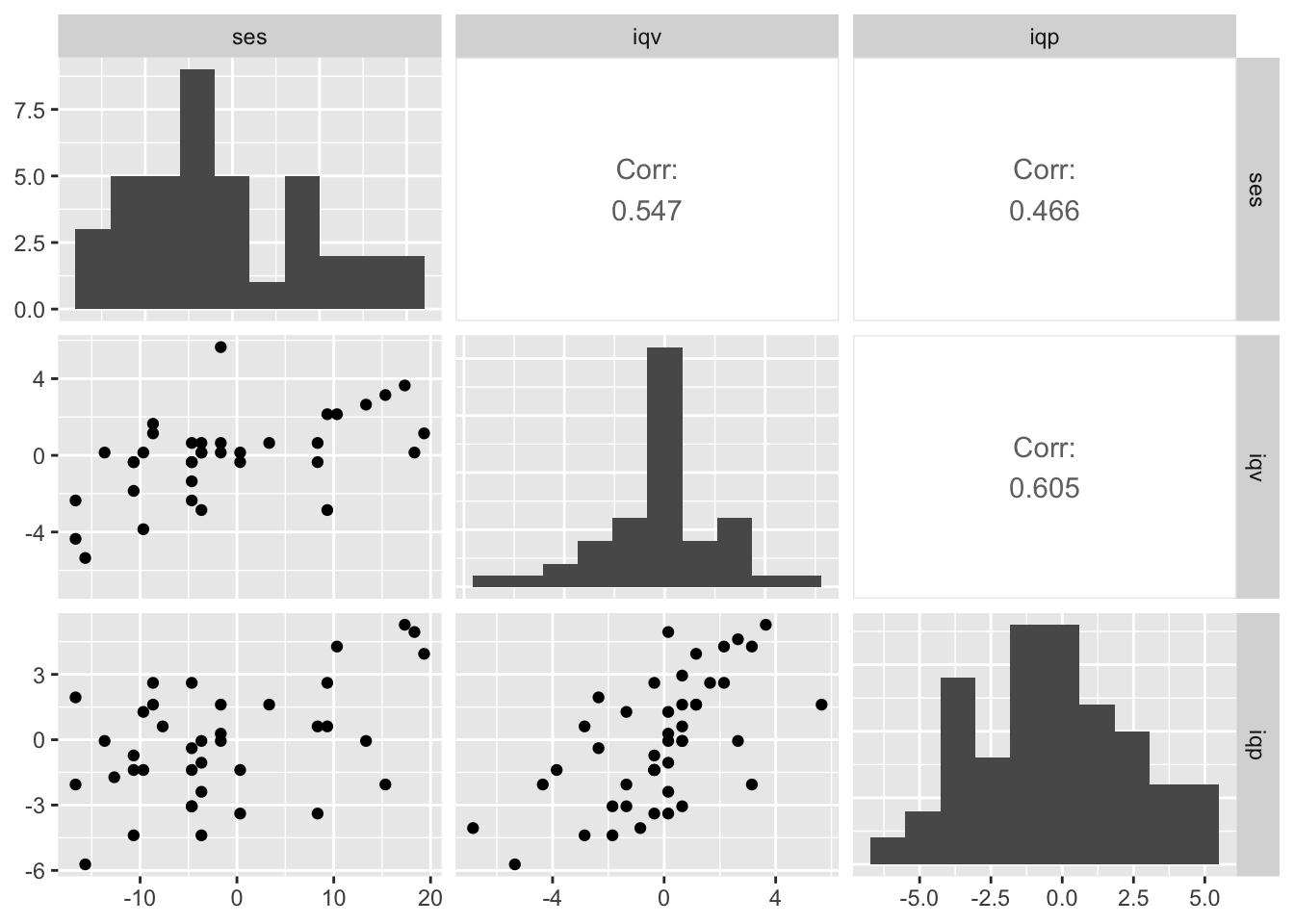
We’ll be focusing on the relation between socioeconomic status (ses) and verbal IQ (iqv) and performance IQ (iqp) will be a missing data covariate.

Here’s what the missing data patterns look like.

b_small %>% 
  mutate_all(.funs = ~ ifelse(is.na(.), 0, 1)) %>% 
  count(ses, iqv, iqp, sort = TRUE) %>% 
  mutate(percent = 100 * n / sum(n))

##   ses iqv iqp  n percent
## 1   1   1   1 36      72
## 2   0   1   1 11      22
## 3   1   0   1  2       4
## 4   1   0   0  1       2

Here 1 means the value was observed and 0 means the value was missing. Twenty-eight percent of the cases have missingness on one of the two focal variables. The bulk of the missingness is in ses.

Impute

We’ll use the mice() function to impute. By setting m = 10, we’ll get back 10 multiply-imputed data sets. By setting method = "norm", we will be using Bayesian linear regression with the Gaussian likelihood to compute the imputed values.

imp <- mice(b_small, seed = 540, m = 10, method = "norm", print = FALSE)

Model

Our statistical model will be

$$ \begin{align*} \text{iqv}_i & \sim \mathcal N(\mu_i, \sigma) \\ \mu_i & = \beta_0 + \beta_1 \text{ses}_i. \end{align*} $$

With the mice::with() function, we fit that model once to each of the 10 imputed data sets.

fit <- with(imp, lm(iqv ~ 1 + ses))

There’s a lot of information packed into our fit object. Within the analyses section we can find the results of all 10 models.

fit$analyses %>% str(max.level = 1)

## List of 10
##  $ :List of 12
##   ..- attr(*, "class")= chr "lm"
##  $ :List of 12
##   ..- attr(*, "class")= chr "lm"
##  $ :List of 12
##   ..- attr(*, "class")= chr "lm"
##  $ :List of 12
##   ..- attr(*, "class")= chr "lm"
##  $ :List of 12
##   ..- attr(*, "class")= chr "lm"
##  $ :List of 12
##   ..- attr(*, "class")= chr "lm"
##  $ :List of 12
##   ..- attr(*, "class")= chr "lm"
##  $ :List of 12
##   ..- attr(*, "class")= chr "lm"
##  $ :List of 12
##   ..- attr(*, "class")= chr "lm"
##  $ :List of 12
##   ..- attr(*, "class")= chr "lm"

This insight will come in handy in just a bit.

We want lines!

Start naïve.

If you wanted to plot the fitted line for a simple linear model, you’d probably use the fitted() or predict() function. But when you have fit that model to your multiply-imputed data sets, that just won’t work. For example:

predict(fit)

If you try executing that line, you’ll get a nasty error message reading:

Error in UseMethod(“predict”) : no applicable method for ‘predict’ applied to an object of class “c(‘mira’, ‘matrix’)”

Our fit object is not a regular fit object. It’s an object of class "mira" and "matrix", which means it’s fancy and temperamental.

class(fit)

## [1] "mira"   "matrix"

At the time of this writing, the mice package does not have a built-in solution to this problem. If you’re willing to put in a little work, you can do the job yourself.

Off label.

Remember how we showed how our fit$analyses is a list of all 10 of our individual model fits? Turns out we can leverage that. For example, here’s the model summary for the model fit to the seventh imputed data set.

fit$analyses[[7]] %>% 
  summary()

## 
## Call:
## lm(formula = iqv ~ 1 + ses)
## 
## Residuals:
##     Min      1Q  Median      3Q     Max 
## -4.1947 -1.0600  0.1209  0.9678  5.5680 
## 
## Coefficients:
##             Estimate Std. Error t value Pr(>|t|)    
## (Intercept)  0.26981    0.29403   0.918 0.363405    
## ses          0.11479    0.02732   4.201 0.000115 ***
## ---
## Signif. codes:  0 '***' 0.001 '**' 0.01 '*' 0.05 '.' 0.1 ' ' 1
## 
## Residual standard error: 2.024 on 48 degrees of freedom
## Multiple R-squared:  0.2689, Adjusted R-squared:  0.2536 
## F-statistic: 17.65 on 1 and 48 DF,  p-value: 0.0001146

All we needed to do was use the double-bracket indexing. If you’re not up on how to do that, Hadley Wickham has a famous tweet on the subject and Jenny Bryan has a great talk discussing the role of lists within data wrangling. With the double-bracket indexing trick, you can use fitted() or predict() one model iteration at a time. E.g.,

fit$analyses[[1]] %>% 
  fitted() %>% 
  str()

##  Named num [1:50] -1.341 0.135 -0.512 1.975 -0.794 ...
##  - attr(*, "names")= chr [1:50] "1" "2" "3" "4" ...

Building, here’s what that can look like if we use predict() for all 10 of our models, bind the individual results, and plot them all at once.

# define the sequence of predictor values
ses_min <- min(b_small$ses, na.rm = T)
ses_max <- max(b_small$ses, na.rm = T)

ses_length <- 30

nd <- tibble(ses = seq(from = ses_min, to = ses_max, length.out = ses_length))

# use `predict()` for each separate model
rbind(
  predict(fit$analyses[[1]], newdata = nd, interval = "confidence"),
  predict(fit$analyses[[2]], newdata = nd, interval = "confidence"),
  predict(fit$analyses[[3]], newdata = nd, interval = "confidence"),
  predict(fit$analyses[[4]], newdata = nd, interval = "confidence"),
  predict(fit$analyses[[5]], newdata = nd, interval = "confidence"),
  predict(fit$analyses[[6]], newdata = nd, interval = "confidence"),
  predict(fit$analyses[[7]], newdata = nd, interval = "confidence"),
  predict(fit$analyses[[8]], newdata = nd, interval = "confidence"),
  predict(fit$analyses[[9]], newdata = nd, interval = "confidence"),
  predict(fit$analyses[[10]], newdata = nd, interval = "confidence")
) %>%
  # wrangle a bit
  data.frame() %>% 
  bind_cols(
    bind_rows(replicate(10, nd, simplify = FALSE))
    ) %>% 
  mutate(.imp = rep(1:10, each = ses_length)) %>% 
  
  # plot!
  ggplot(aes(x = ses)) +
  geom_ribbon(aes(ymin = lwr, ymax = upr, group = .imp),
              alpha = 1/10) +
  geom_line(aes(y = fit, group = .imp), 
            size = 1/4) +
  # add the observed data for good measure
  geom_point(data = b_small,
             aes(y = iqv)) +
  ylab("iqv")

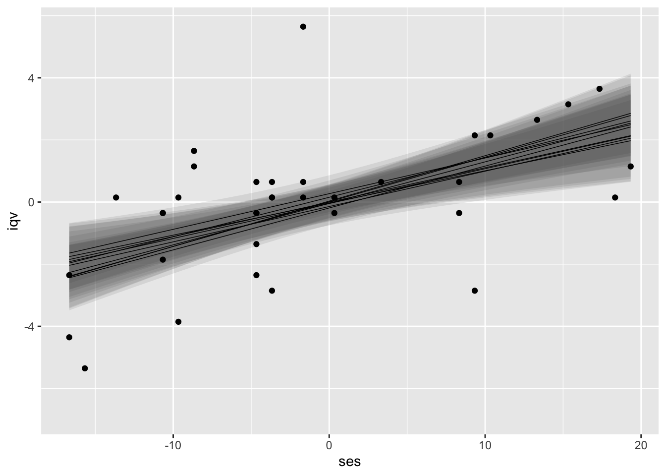
I kinda like this visualization approach. It has a certain Bayesian flair and it does an okay job displaying the stochasticity built in to the multiple imputation framework. However, this approach is totally off label and will probably get shot down by any self-respecting Reviewer #2.

Fortunately for us, we have a principled and peer-reviewed solution, instead.

Level up with Miles.

In his ( 2016) paper, Obtaining predictions from models fit to multiply imputed data, Andrew Miles presented two methods for, well, doing what his title said he’d do. Miles called these two methods Predict Then Combine (PC) and Combine Then Predict (CP). The CP approach invokes first derivatives in a way I’m not prepared to implement on my own. Fortunately for us, the PC approach just requires a little iteration, a few lines within a grouped summarise(), and a tiny bit of wrangling. In my world, that’s cake. 🍰

First: iteration.

For our first step, we’ll use predict() again for each of our individual versions of the model. This time, however, we’ll use thriftier code and iterate with help from purrr::map().

fitted_lines <-
  tibble(.imp = 1:10) %>% 
  mutate(p = map(.imp, ~ predict(fit$analyses[[.]], 
                                 newdata = nd, 
                                 se.fit = TRUE) %>% 
                   data.frame())
         )

# what have we done?
fitted_lines

## # A tibble: 10 × 2
##     .imp p            
##    <int> <list>       
##  1     1 <df [30 × 4]>
##  2     2 <df [30 × 4]>
##  3     3 <df [30 × 4]>
##  4     4 <df [30 × 4]>
##  5     5 <df [30 × 4]>
##  6     6 <df [30 × 4]>
##  7     7 <df [30 × 4]>
##  8     8 <df [30 × 4]>
##  9     9 <df [30 × 4]>
## 10    10 <df [30 × 4]>

We have a nested tibble where the results of all 10 predict() operations are waiting for us in the p column and each is conveniently indexed by .imp. Note also how we did not request confidence intervals in the output, but we did set se.fit = TRUE. We’ll be all about those standard errors in just a bit.

Here’s how we unnest the results and then augment a little.

fitted_lines <- fitted_lines %>% 
  unnest(p) %>% 
  # add in the nd predictor data
  bind_cols(
    bind_rows(replicate(10, nd, simplify = FALSE))
    ) %>% 
  # drop two unneeded columns
  select(-df, -residual.scale)

# now what did we do?
glimpse(fitted_lines)

## Rows: 300
## Columns: 4
## $ .imp   <int> 1, 1, 1, 1, 1, 1, 1, 1, 1, 1, 1, 1, 1, 1, 1, 1, 1, 1, 1, 1, 1, …
## $ fit    <dbl> -1.75590067, -1.62725529, -1.49860992, -1.36996455, -1.24131917…
## $ se.fit <dbl> 0.5285145, 0.4991145, 0.4705449, 0.4429666, 0.4165764, 0.391614…
## $ ses    <dbl> -16.6666667, -15.4252874, -14.1839080, -12.9425287, -11.7011494…

Second: equations and the implied code.

In his paper (p. 176), Miles’s used predictions

as a blanket term for any value \(\hat p\) that can be calculated by applying some type of transformation \(t()\) to the vector of coefficients from a fitted model \((\hat \beta)\).

$$\hat p = t(\hat \beta)$$

In our case, \(\hat p\) covers the values in our fit column and the \(t(\hat \beta)\) part is what we did with predict(). Well, technically we should refer to those fit values as \(\hat p_j\), where \(j\) is the index for a given imputed data set, \(j = 1, \dots, m\), and \(m\) is the total number of imputations. In our fitted_lines tibble, we have called Miles’s \(m\) index .imp².

Anyway, Miles showed we can compute the conditional pooled point estimate \(\bar p\) by

$$\bar p = \frac{1}{m} \sum_{j=1}^m \hat p_j,$$

which is a formal way of saying we simply average across the \(m\) imputed solutions. Here’s that in code.

fitted_lines %>% 
  group_by(ses) %>% 
  summarise(fit_bar = mean(fit))

## # A tibble: 30 × 2
##       ses fit_bar
##     <dbl>   <dbl>
##  1 -16.7   -2.07 
##  2 -15.4   -1.91 
##  3 -14.2   -1.76 
##  4 -12.9   -1.60 
##  5 -11.7   -1.45 
##  6 -10.5   -1.30 
##  7  -9.22  -1.14 
##  8  -7.98  -0.989
##  9  -6.74  -0.835
## 10  -5.49  -0.681
## # … with 20 more rows

Though the expected values are pretty easy to compute, it’ll take a little more effort to express the uncertainty around those expectations because we have to account for both within- and between-imputation variance. We can define the within-imputation variance \(V_W\) as

$$V_W = \frac{1}{m} \sum_{j=1}^m \widehat{SE}_j^2,$$

which is a formal way of saying we simply average the squared standard errors across the \(m\) imputed solutions, for each fitted value. Here’s that in code.

fitted_lines %>% 
  group_by(ses) %>% 
  summarise(fit_bar = mean(fit),
            v_w     = mean(se.fit^2))

## # A tibble: 30 × 3
##       ses fit_bar    v_w
##     <dbl>   <dbl>  <dbl>
##  1 -16.7   -2.07  0.260 
##  2 -15.4   -1.91  0.232 
##  3 -14.2   -1.76  0.206 
##  4 -12.9   -1.60  0.182 
##  5 -11.7   -1.45  0.161 
##  6 -10.5   -1.30  0.142 
##  7  -9.22  -1.14  0.126 
##  8  -7.98  -0.989 0.112 
##  9  -6.74  -0.835 0.100 
## 10  -5.49  -0.681 0.0908
## # … with 20 more rows

We can define the between imputation variance \(V_B\) as

$$V_B = \frac{1}{m - 1} \sum_{j=1}^m (\hat p_j - \bar p_j)^2,$$

where we’re no longer quite averaging across the \(m\) imputations because our denominator is now the corrected value \((m - 1)\). What can I say? Variances are tricky. Here’s the code.

# define the total number of imputations
m <- 10

fitted_lines %>% 
  group_by(ses) %>% 
  summarise(fit_bar = mean(fit),
            v_w     = mean(se.fit^2),
            v_b     = sum((fit - fit_bar)^2) / (m - 1))

## # A tibble: 30 × 4
##       ses fit_bar    v_w    v_b
##     <dbl>   <dbl>  <dbl>  <dbl>
##  1 -16.7   -2.07  0.260  0.0833
##  2 -15.4   -1.91  0.232  0.0742
##  3 -14.2   -1.76  0.206  0.0657
##  4 -12.9   -1.60  0.182  0.0579
##  5 -11.7   -1.45  0.161  0.0508
##  6 -10.5   -1.30  0.142  0.0444
##  7  -9.22  -1.14  0.126  0.0387
##  8  -7.98  -0.989 0.112  0.0336
##  9  -6.74  -0.835 0.100  0.0293
## 10  -5.49  -0.681 0.0908 0.0256
## # … with 20 more rows

We can define the total variance of the prediction \(V_{\bar p}\) as

$$V_{\bar p} = V_W + V_B \left ( 1 + \frac{1}{m} \right ),$$

where the pooled standard error is just \(\sqrt{V_{\bar p}}\). Here are those in code.

fitted_lines %>% 
  group_by(ses) %>% 
  summarise(fit_bar = mean(fit),
            v_w     = mean(se.fit^2),
            v_b     = sum((fit - fit_bar)^2) / (m - 1),
            v_p     = v_w + v_b * (1 + (1 / m)),
            se_p    = sqrt(v_p))

## # A tibble: 30 × 6
##       ses fit_bar    v_w    v_b   v_p  se_p
##     <dbl>   <dbl>  <dbl>  <dbl> <dbl> <dbl>
##  1 -16.7   -2.07  0.260  0.0833 0.352 0.593
##  2 -15.4   -1.91  0.232  0.0742 0.313 0.560
##  3 -14.2   -1.76  0.206  0.0657 0.278 0.527
##  4 -12.9   -1.60  0.182  0.0579 0.246 0.496
##  5 -11.7   -1.45  0.161  0.0508 0.217 0.465
##  6 -10.5   -1.30  0.142  0.0444 0.191 0.437
##  7  -9.22  -1.14  0.126  0.0387 0.168 0.410
##  8  -7.98  -0.989 0.112  0.0336 0.149 0.385
##  9  -6.74  -0.835 0.100  0.0293 0.132 0.364
## 10  -5.49  -0.681 0.0908 0.0256 0.119 0.345
## # … with 20 more rows

Now we finally have both \(\bar p\) and \(V_{\bar p}\) for each desired level of ses, we can use the conventional normal-theory approach to compute the pooled 95% confidence intervals.

# this time we'll save the results
fitted_lines <- fitted_lines %>% 
  group_by(ses) %>% 
  summarise(fit_bar = mean(fit),
            v_w     = mean(se.fit^2),
            v_b     = sum((fit - fit_bar)^2) / (m - 1),
            v_p     = v_w + v_b * (1 + (1 / m)),
            se_p    = sqrt(v_p)) %>% 
  # use the _p suffix to indicate these are pooled
  mutate(lwr_p = fit_bar - se_p * 1.96,
         upr_p = fit_bar + se_p * 1.96) 

# what do we have?
glimpse(fitted_lines)

## Rows: 30
## Columns: 8
## $ ses     <dbl> -16.6666667, -15.4252874, -14.1839080, -12.9425287, -11.701149…
## $ fit_bar <dbl> -2.06663732, -1.91265660, -1.75867587, -1.60469515, -1.4507144…
## $ v_w     <dbl> 0.25989881, 0.23153126, 0.20555857, 0.18198075, 0.16079779, 0.…
## $ v_b     <dbl> 0.08332943, 0.07416123, 0.06568224, 0.05789246, 0.05079188, 0.…
## $ v_p     <dbl> 0.35156118, 0.31310861, 0.27780903, 0.24566245, 0.21666886, 0.…
## $ se_p    <dbl> 0.5929259, 0.5595611, 0.5270759, 0.4956435, 0.4654770, 0.43683…
## $ lwr_p   <dbl> -3.22877218, -3.00939633, -2.79174469, -2.57615635, -2.3630493…
## $ upr_p   <dbl> -0.904502468, -0.815916869, -0.725607057, -0.633233949, -0.538…

Third: plot.

Now the hard part is over, we’re finally ready to plot.

fitted_lines %>% 
  ggplot(aes(x = ses)) +
  geom_ribbon(aes(ymin = lwr_p, ymax = upr_p),
              alpha = 1/2) +
  geom_line(aes(y = fit_bar), 
            size = 1/2) +
  # add the observed data for good measure
  geom_point(data = b_small,
             aes(y = iqv)) +
  labs(title = "Pooled fitted line from a model fit to multiply-imputed data",
       subtitle = expression("The pooled conditional mean line "*(bar(italic(p)))*" sits atop the pooled confidence interval "*(95*'%'*~CI[bar(italic(p))])*' band.'),
       y = "iqv")

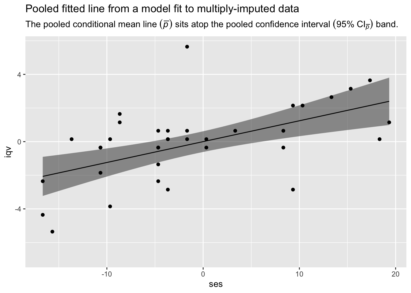
There it is, friends. We have the pooled fitted line and its pooled 95% confidence interval band from our model fit to multiply-imputed data. Until the day that Stef van Buuren and friends get around to building this functionality into mice, our realization in R code of Andrew Miles’s Predict Then Combine (PC) approach has you covered.

Session info

sessionInfo()

## R version 4.2.0 (2022-04-22)
## Platform: x86_64-apple-darwin17.0 (64-bit)
## Running under: macOS Big Sur/Monterey 10.16
## 
## Matrix products: default
## BLAS:   /Library/Frameworks/R.framework/Versions/4.2/Resources/lib/libRblas.0.dylib
## LAPACK: /Library/Frameworks/R.framework/Versions/4.2/Resources/lib/libRlapack.dylib
## 
## locale:
## [1] en_US.UTF-8/en_US.UTF-8/en_US.UTF-8/C/en_US.UTF-8/en_US.UTF-8
## 
## attached base packages:
## [1] stats     graphics  grDevices utils     datasets  methods   base     
## 
## other attached packages:
##  [1] mice_3.14.0     GGally_2.1.2    forcats_0.5.1   stringr_1.4.1  
##  [5] dplyr_1.0.10    purrr_0.3.4     readr_2.1.2     tidyr_1.2.1    
##  [9] tibble_3.1.8    ggplot2_3.4.0   tidyverse_1.3.2
## 
## loaded via a namespace (and not attached):
##  [1] Rcpp_1.0.9          lattice_0.20-45     lubridate_1.8.0    
##  [4] assertthat_0.2.1    digest_0.6.30       utf8_1.2.2         
##  [7] plyr_1.8.7          R6_2.5.1            cellranger_1.1.0   
## [10] backports_1.4.1     reprex_2.0.2        evaluate_0.18      
## [13] highr_0.9           httr_1.4.4          blogdown_1.15      
## [16] pillar_1.8.1        rlang_1.0.6         googlesheets4_1.0.1
## [19] readxl_1.4.1        rstudioapi_0.13     jquerylib_0.1.4    
## [22] rmarkdown_2.16      labeling_0.4.2      googledrive_2.0.0  
## [25] munsell_0.5.0       broom_1.0.1         compiler_4.2.0     
## [28] modelr_0.1.8        xfun_0.35           pkgconfig_2.0.3    
## [31] htmltools_0.5.3     tidyselect_1.1.2    bookdown_0.28      
## [34] emo_0.0.0.9000      reshape_0.8.9       fansi_1.0.3        
## [37] crayon_1.5.2        tzdb_0.3.0          dbplyr_2.2.1       
## [40] withr_2.5.0         grid_4.2.0          jsonlite_1.8.3     
## [43] gtable_0.3.1        lifecycle_1.0.3     DBI_1.1.3          
## [46] magrittr_2.0.3      scales_1.2.1        cli_3.4.1          
## [49] stringi_1.7.8       cachem_1.0.6        farver_2.1.1       
## [52] fs_1.5.2            xml2_1.3.3          bslib_0.4.0        
## [55] ellipsis_0.3.2      generics_0.1.3      vctrs_0.5.0        
## [58] RColorBrewer_1.1-3  tools_4.2.0         glue_1.6.2         
## [61] hms_1.1.1           fastmap_1.1.0       yaml_2.3.5         
## [64] colorspace_2.0-3    gargle_1.2.0        rvest_1.0.2        
## [67] knitr_1.40          haven_2.5.1         sass_0.4.2

References

Brandsma, H., & Knuver, J. (1989). Effects of school and classroom characteristics on pupil progress in language and arithmetic. International Journal of Educational Research, 13(7), 777–788. https://doi.org/10.1016/0883-0355(89)90028-1
Enders, C. K. (2022). Applied missing data analysis (Second Edition). Guilford Press. http://www.appliedmissingdata.com/
Gelman, A., Hill, J., & Vehtari, A. (2020). Regression and other stories. Cambridge University Press. https://doi.org/10.1017/9781139161879
James, G., Witten, D., Hastie, T., & Tibshirani, R. (2021). An introduction to statistical learning with applications in R (Second Edition). Springer. https://web.stanford.edu/~hastie/ISLRv2_website.pdf
Kruschke, J. K. (2015). Doing Bayesian data analysis: A tutorial with R, JAGS, and Stan. Academic Press. https://sites.google.com/site/doingbayesiandataanalysis/
Little, R. J., & Rubin, D. B. (2019). Statistical analysis with missing data (3rd ed., Vol. 793). John Wiley & Sons. https://www.wiley.com/en-us/Statistical+Analysis+with+Missing+Data%2C+3rd+Edition-p-9780470526798
McElreath, R. (2015). Statistical rethinking: A Bayesian course with examples in R and Stan. CRC press. https://xcelab.net/rm/statistical-rethinking/
McElreath, R. (2020). Statistical rethinking: A Bayesian course with examples in R and Stan (Second Edition). CRC Press. https://xcelab.net/rm/statistical-rethinking/
Miles, A. (2016). Obtaining predictions from models fit to multiply imputed data. Sociological Methods & Research, 45(1), 175–185. https://doi.org/10.1177/0049124115610345
R Core Team. (2022). R: A language and environment for statistical computing. R Foundation for Statistical Computing. https://www.R-project.org/
Roback, P., & Legler, J. (2021). Beyond multiple linear regression: Applied generalized linear models and multilevel models in R. CRC Press. https://bookdown.org/roback/bookdown-BeyondMLR/
Schloerke, B., Crowley, J., Di Cook, Briatte, F., Marbach, M., Thoen, E., Elberg, A., & Larmarange, J. (2021). GGally: Extension to ’ggplot2’. https://CRAN.R-project.org/package=GGally
van Buuren, S. (2018). Flexible imputation of missing data (Second Edition). CRC Press. https://stefvanbuuren.name/fimd/
van Buuren, S., & Groothuis-Oudshoorn, K. (2011). mice: Multivariate imputation by chained equations in R. Journal of Statistical Software, 45(3), 1–67. https://www.jstatsoft.org/v45/i03/
van Buuren, S., & Groothuis-Oudshoorn, K. (2021). mice: Multivariate imputation by chained equations [Manual]. https://CRAN.R-project.org/package=mice
Wickham, H. (2022). tidyverse: Easily install and load the ’tidyverse’. https://CRAN.R-project.org/package=tidyverse
Wickham, H., Averick, M., Bryan, J., Chang, W., McGowan, L. D., François, R., Grolemund, G., Hayes, A., Henry, L., Hester, J., Kuhn, M., Pedersen, T. L., Miller, E., Bache, S. M., Müller, K., Ooms, J., Robinson, D., Seidel, D. P., Spinu, V., … Yutani, H. (2019). Welcome to the tidyverse. Journal of Open Source Software, 4(43), 1686. https://doi.org/10.21105/joss.01686
-
Be warned that “full-luxury Bayesian …” isn’t a real term. Rather, it’s a playful descriptor coined by the great Richard McElreath. To hear him use it in action, check out his nifty talk on causal inference. One-step Bayesian imputation is a real thing, though. McElreath covered it in both editions of his text and I’ve even blogged about it here. ↩︎
When you do this on your own, you might instead name the
.impcolumn asm, which goes nicely with Miles’s notation. In this post and in some of my personal work, I used.impbecause it lines up nicely with the output from some of the mice functions. ↩︎
- Posted on:
- October 21, 2021
- Length:
- 17 minute read, 3548 words