One-step Bayesian imputation when you have dropout in your RCT

Version 1.1.0

Edited on December 12, 2022, to use the new as_draws_df() workflow.

Preamble

Suppose you’ve got data from a randomized controlled trial (RCT) where participants received either treatment or control. Further suppose you only collected data at two time points, pre- and post-treatment. Even in the best of scenarios, you’ll probably have some dropout in those post-treatment data. To get the full benefit of your data, you can use one-step Bayesian imputation when you compute your effect sizes. In this post, I’ll show you how.

I make assumptions.

For this post, I’m presuming you have a passing familiarity with the following:

• You should be familiar with effect sizes, particularly with standardized mean differences. If you need to brush up, consider Cohen’s ( 1988) authoritative text, or Cummings newer ( 2012) text. For nice conceptual overview, I also recommend Kelley and Preacher’s ( 2012) paper, On effect size.

• You should be familiar with Bayesian regression. For thorough introductions, I recommend either edition of McElreath’s text ( 2020, 2015); Kruschke’s ( 2015) text; or Gelman, Hill, and Vehtari’s ( 2020) text. If you go with McElreath, he has a fine series of freely-available lectures here.

• Though we won’t be diving deep into it, here, you’ll want to have some familiarity with contemporary missing data theory. You can find brief overviews in the texts by McElreath and Gelman et al, above. For a deeper dive, I recommend Enders ( 2010) or Little & Rubin ( 2019). Also, heads up: word on the street is Enders is working on a second edition of his book.

• All code is in R ( R Core Team, 2022). Data wrangling and plotting were done with help from the tidyverse ( Wickham et al., 2019; Wickham, 2022) and tidybayes ( Kay, 2022). The data were simulated with help from the faux package ( DeBruine, 2021) and the Bayesian models were fit using brms ( Bürkner, 2017, 2018, 2022).

Here we load our primary R packages and adjust the global plotting theme defaults.

library(tidyverse)
library(faux)
library(tidybayes)
library(brms)

# adjust the global plotting theme
theme_set(
  theme_tidybayes() +
    theme(axis.line.x = element_blank(),
          axis.line.y = element_blank(),
          panel.border = element_rect(color = "grey85", linewidth = 1, fill = NA))
)

We need data.

For this post, we’ll be simulating our data with help from the handy faux::rnorm_multi() function. To start out, we’ll make two data sets, one for treatment (d_treatment) and one for control (d_control). Each will contain outcomes at pre and post treatment, with the population parameters for both conditions at pre being \(\operatorname{Normal}(5, 1)\). Whereas those parameters stay the same at post for those in the control condition, the population parameters for those in the treatment condition will raise at post to \(\operatorname{Normal}(5.7, 1)\). Notice that not only did their mean value increase, but their standard deviation increased a bit, too, which is not uncommon in treatment data. Importantly, the correlation between pre and post is \(.75\) for both conditions.

# how many per group?
n <- 100

set.seed(1)

d_treatment <- rnorm_multi(
  n = n,
  mu = c(5, 5.7),
  sd = c(1, 1.1), 
  r = .75, 
  varnames = list("pre", "post")
)

d_control <- rnorm_multi(
  n = n,
  mu = c(5, 5),
  sd = c(1, 1), 
  r = .75, 
  varnames = list("pre", "post")
)

Next we combine the two data sets and make an explicit tx variable to distinguish the conditions. Then we simulate missingness in the post variable in two steps: We use the rbinom() function to simulate whether a case will be missing and then use a little ifelse() to make a post_observed variable that is the same as post except that the vales are missing in every row for which missing == 1.

set.seed(1)

d <- bind_rows(
  d_control,
  d_treatment
) %>% 
  mutate(tx = rep(c("control", "treatment"), each = n)) %>% 
  mutate(tx = factor(tx, levels = c("treatment", "control"))) %>% 
  mutate(missing = rbinom(n(), size = 1, prob = 0.3)) %>%
  mutate(post_observed = ifelse(missing == 1, NA, post))

head(d)

##        pre     post      tx missing post_observed
## 1 5.066999 5.698922 control       0      5.698922
## 2 6.950072 6.209520 control       0      6.209520
## 3 5.787145 7.181091 control       0      7.181091
## 4 4.826099 4.554830 control       1            NA
## 5 2.277529 3.447187 control       0      3.447187
## 6 6.801701 7.870996 control       1            NA

To get a sense for the data, here’s a scatter plot of pre versus post, by tx and missing.

d %>% 
  mutate(missing = factor(missing,
                          levels = 1:0,
                          labels = c("yes", "no"))) %>% 
  
  ggplot(aes(x = pre, y = post, color = missing, shape = missing)) +
  geom_point() +
  scale_color_viridis_d(option = "D", begin = .35, end = .75, direction = -1) +
  scale_shape_manual(values = 17:16) +
  coord_equal(xlim = c(1.5, 8.5),
              ylim = c(1.5, 8.5)) +
  facet_wrap(~ tx)

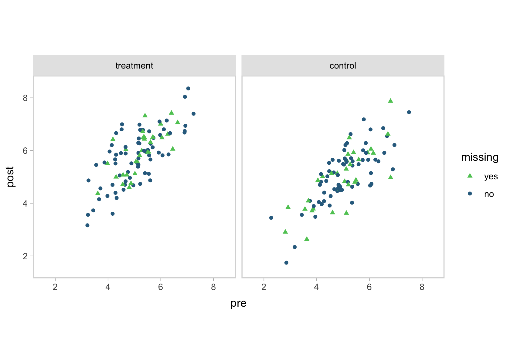
You can see that high correlation between pre and post in the shapes of the data clouds. To look at the data in another way, here are a few summary statistics.

d %>% 
  pivot_longer(starts_with("p"), names_to = "time") %>% 
  mutate(time = factor(time, levels = c("pre", "post", "post_observed"))) %>% 
  group_by(tx, time) %>% 
  summarise(mean = mean(value, na.rm = T),
            sd = sd(value, na.rm = T),
            min = min(value, na.rm = T),
            max = max(value, na.rm = T)) %>% 
  mutate_if(is.double, round, digits = 2)

## # A tibble: 6 × 6
## # Groups:   tx [2]
##   tx        time           mean    sd   min   max
##   <fct>     <fct>         <dbl> <dbl> <dbl> <dbl>
## 1 treatment pre            5.11  0.91  3.22  7.24
## 2 treatment post           5.8   0.99  3.16  8.35
## 3 treatment post_observed  5.74  1.05  3.16  8.35
## 4 control   pre            5.01  0.99  2.28  7.5 
## 5 control   post           5.05  1.06  1.74  7.87
## 6 control   post_observed  5.1   1.04  1.74  7.45

Statistical models

We’ll be analyzing the RCT data in two ways. First, we’ll fit a model on the version of the data with no missingness in post. That will be our benchmark. Then we’ll practice fitting the model with one-step Bayesian imputation and the post_observed variable. Once we’ve fit and evaluated our models, we’ll then walk out how to compute the effect sizes.

Fit the models.

There are a lot of ways to analyze pre/post RCT data. To get a sense of the various strategies, see this chapter in Jeffrey Walker’s free ( 2018) text and my complimentary blog post on pre/post non-experimental data. In this post, we’ll be taking the multivariate approach where we simultaneously model pre and post as bivariate normal, such that both the mean and standard deviation parameters for both vary depending on the experimental condition (tx). Importantly, the correlation between pre and post is captured in the correlation between the two residual standard deviation parameters.

Here’s how to fit the model to the full data with brms.

fit1 <- brm(
  data = d,
  family = gaussian,
  bf(pre ~ 0 + tx, sigma ~ 0 + tx) +
    bf(post ~ 0 + tx, sigma ~ 0 + tx) +
    set_rescor(rescor = TRUE),
  prior = c(prior(normal(5, 1), class = b, resp = pre),
            prior(normal(5, 1), class = b, resp = post),
            prior(normal(log(1), 1), class = b, dpar = sigma, resp = pre),
            prior(normal(log(1), 1), class = b, dpar = sigma, resp = post),
            prior(lkj(2), class = rescor)),
  cores = 4,
  seed = 1
)

The priors in this post follow the weakly-regularizing approach McElreath advocated for in the second edition of this text. Also note that because we are allowing the residual standard deviation parameter to vary by tx, the brms default is to use the log link, which will become important for interpretation and post processing. Here’s the parameter summary.

print(fit1)

##  Family: MV(gaussian, gaussian) 
##   Links: mu = identity; sigma = log
##          mu = identity; sigma = log 
## Formula: pre ~ 0 + tx 
##          sigma ~ 0 + tx
##          post ~ 0 + tx 
##          sigma ~ 0 + tx
##    Data: d (Number of observations: 200) 
##   Draws: 4 chains, each with iter = 2000; warmup = 1000; thin = 1;
##          total post-warmup draws = 4000
## 
## Population-Level Effects: 
##                        Estimate Est.Error l-95% CI u-95% CI Rhat Bulk_ESS Tail_ESS
## pre_txtreatment            5.00      0.10     4.81     5.19 1.00     2801     3091
## pre_txcontrol              5.11      0.09     4.93     5.29 1.00     3300     2885
## sigma_pre_txtreatment     -0.03      0.06    -0.15     0.09 1.00     3700     3273
## sigma_pre_txcontrol       -0.08      0.07    -0.21     0.06 1.00     3536     3105
## post_txtreatment           5.74      0.11     5.52     5.96 1.00     3027     2940
## post_txcontrol             5.08      0.09     4.90     5.26 1.00     3306     2758
## sigma_post_txtreatment     0.14      0.06     0.02     0.27 1.00     3555     3230
## sigma_post_txcontrol      -0.08      0.07    -0.21     0.05 1.00     3608     2764
## 
## Residual Correlations: 
##                  Estimate Est.Error l-95% CI u-95% CI Rhat Bulk_ESS Tail_ESS
## rescor(pre,post)     0.73      0.03     0.67     0.79 1.00     3476     3305
## 
## Draws were sampled using sampling(NUTS). For each parameter, Bulk_ESS
## and Tail_ESS are effective sample size measures, and Rhat is the potential
## scale reduction factor on split chains (at convergence, Rhat = 1).

After exponentiating the standard deviations, all the parameter summaries look close to the data generating values from our faux::rnorm_multi() code. This, however, is all just a warm-up. Our goal was to use one-step Bayesian imputation for when we have missing data at post-intervention time point. From a syntax perspective, that involves a few minor changes to our fit1 code. First, we replace the post variable with post_observed, which had about \(30\%\) of the values missing. In a similar way, we have to adjust a few of the resp arguments within the prior() statements. Finally and most crucially, we have to include the | mi() syntax when defining the linear model for post_observed. Otherwise, brms will simply drop all the cases with missingness on post_observed.

Here’s the code.

fit2 <- brm(
  data = d,
  family = gaussian,
  bf(pre ~ 0 + tx,
     sigma ~ 0 + tx) +
    # notice the changes in this line
    bf(post_observed | mi() ~ 0 + tx,
       sigma ~ 0 + tx) +
    set_rescor(rescor = TRUE),
  prior = c(prior(normal(5, 1), class = b, resp = pre),
            # notice the changes in the `resp` argument
            prior(normal(5, 1), class = b, resp = postobserved),
            prior(normal(log(1), 1), class = b, dpar = sigma, resp = pre),
            # notice the changes in the `resp` argument
            prior(normal(log(1), 1), class = b, dpar = sigma, resp = postobserved),
            prior(lkj(2), class = rescor)),
  cores = 4,
  seed = 1
)

Instead of looking at the print() output, it might be more informative if we compare the results of our two models in a coefficient plot.

# define the parameter names
parameters <- c(
  "mu[treatment]^pre", "mu[control]^pre", "sigma[treatment]^pre", "sigma[control]^pre",
  "mu[treatment]^post", "mu[control]^post", "sigma[treatment]^post", "sigma[control]^post", 
  "rho"
  )

# define the deisred order for the parameter names
levels <- c(
  "mu[treatment]^pre", "mu[control]^pre", "mu[treatment]^post", "mu[control]^post", 
  "sigma[treatment]^pre", "sigma[control]^pre", "sigma[treatment]^post", "sigma[control]^post", 
  "rho"
  )

# combine the posterior summaries for the two models
rbind(
  posterior_summary(fit1)[1:9, -2],
  posterior_summary(fit2)[1:9, -2]
  ) %>% 
  # wrangle
  data.frame() %>% 
  mutate(data = rep(c("complete data", "30% missing"), each = n() / 2),
         par  = rep(parameters, times = 2)) %>% 
  mutate(par      = factor(par, levels = levels),
         Estimate = ifelse(str_detect(par, "sigma"), exp(Estimate), Estimate),
         Q2.5     = ifelse(str_detect(par, "sigma"), exp(Q2.5), Q2.5),
         Q97.5    = ifelse(str_detect(par, "sigma"), exp(Q97.5), Q97.5)) %>% 
  
  # plot!
  ggplot(aes(x = Estimate, xmin = Q2.5, xmax = Q97.5, y = data)) +
  geom_pointrange(fatten = 1.1) +
  labs(x = "marginal posterior",
       y = NULL) +
  xlim(0, NA) +
  facet_wrap(~ par, labeller = label_parsed, ncol = 1)

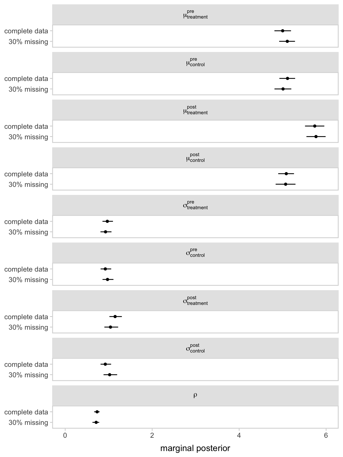
Since the post_observed data were missing completely at random (MCAR¹), it should be no surprise the coefficients are nearly the same between the two models. This, however, will not always (ever?) be the case with your real-world RCT data. Friends, don’t let your friends drop cases or carry the last value forward. Use the brms mi() syntax, instead.

Effect sizes.

At this point, you may be wondering why I didn’t use the familiar dummy-variable approach in either of the models and you might be further wondering why I bothered to allow the standard deviation parameters to vary. One of the sub-goals of this post is to show how to compute the model output into standardized effect sizes. My go-to standardized effect size is good old Cohen’s \(d\), of which there are many variations. In the case of our pre/post RCT with two conditions, we actually have three \(d\)’s of interest:

• the standardized mean difference for the treatment condition (which we hope is large),
• the standardized mean difference for the control condition (which we hope is near zero), and
• the difference in those first two standardized mean differences (which we also hope is large).

As with all standardized mean differences, it’s a big deal to choose a good value to standardize with. With data like ours, a good default choice is the pooled standard deviation between the two conditions at baseline, which we might define as

$$\sigma_p^\text{pre} = \sqrt{\frac{ \left (\sigma_\text{treatment}^\text{pre} \right )^2 + \left (\sigma_\text{control}^\text{pre} \right)^2}{2}},$$

where the notation is admittedly a little verbose. My hope, however, is this notation will make it easier to map the terms onto the model parameters from above. Anyway, with our definition of \(\sigma_p^\text{pre}\) in hand, we’re in good shape to define our three effect sizes of interest as

$$ \begin{align*} d_\text{treatment} & = \frac{\mu_\text{treatment}^\text{post} - \mu_\text{treatment}^\text{pre}}{\sigma_p^\text{pre}}, \\ d_\text{control} & = \frac{\mu_\text{control}^\text{post} - \mu_\text{control}^\text{pre}}{\sigma_p^\text{pre}}, \; \text{and} \\ d_\text{treatment - control} & = \frac{\left ( \mu_\text{treatment}^\text{post} - \mu_\text{treatment}^\text{pre} \right ) - \left ( \mu_\text{control}^\text{post} - \mu_\text{control}^\text{pre} \right )}{\sigma_p^\text{pre}} \\ & = \left (\frac{\mu_\text{treatment}^\text{post} - \mu_\text{treatment}^\text{pre}}{\sigma_p^\text{pre}} \right ) - \left ( \frac{\mu_\text{control}^\text{post} - \mu_\text{control}^\text{pre}}{\sigma_p^\text{pre}} \right ) \\ & = \left ( d_\text{treatment} \right ) - \left ( d_\text{control} \right ). \end{align*} $$

The reason we analyzed the RCT data with a bivariate model with varying means and standard deviations was because the parameter values from that model correspond directly with the various \(\mu\) and \(\sigma\) terms in the equations for \(\sigma_p^\text{pre}\) and our three \(d\)’s. This insight comes from Kruschke ( 2015), particularly Section 16.3. For a walk-through of that section with a brms + tidyverse workflow, see this section of my ebook translation of his text ( Kurz, 2020a). The approach we’re taking, here, is a direct bivariate generalization of the material in Kruschke’s text.

Okay, here’s how to work with the posterior samples from our missing-data model, fit2, to compute those effects.

draws <- as_draws_df(fit2) %>% 
  # exponentiate the log sd parameters
  mutate(`sigma[treatment]^pre` = exp(b_sigma_pre_txtreatment),
         `sigma[control]^pre`   = exp(b_sigma_pre_txcontrol)) %>% 
  # pooled standard deviation (at pre)
  mutate(`sigma[italic(p)]^pre` = sqrt((`sigma[treatment]^pre`^2 + `sigma[control]^pre`^2) / 2)) %>% 
  # within-condition pre/post effect sizes
  mutate(`italic(d)[treatment]` = (b_postobserved_txtreatment - b_pre_txtreatment) / `sigma[italic(p)]^pre`,
         `italic(d)[control]`   = (b_postobserved_txcontrol   - b_pre_txcontrol)   / `sigma[italic(p)]^pre`) %>%
  # between-condition effect size (i.e., difference in differences)
  mutate(`italic(d)['treatment - control']` = `italic(d)[treatment]` - `italic(d)[control]`) 

Now inspect the posteriors for our three \(d\)’s and the \(\sigma_p^\text{pre}\) in a coefficient plot.

levels <- c(
  "sigma[italic(p)]^pre", "italic(d)['treatment - control']", 
  "italic(d)[control]", "italic(d)[treatment]"
  )

draws %>% 
  # wrangle
  pivot_longer(`sigma[italic(p)]^pre`:`italic(d)['treatment - control']`) %>% 
  mutate(parameter = factor(name, levels = levels)) %>% 
  
  # plot
ggplot(aes(x = value, y = parameter)) +
  stat_pointinterval(.width = .95, linewidth = 1/2) +
  scale_y_discrete(labels = ggplot2:::parse_safe) +
  labs(x = "marginal posterior",
       y = NULL) +
  theme(axis.text.y = element_text(hjust = 0),
        axis.ticks.y = element_blank())

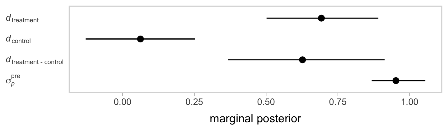
If you look back at the data-generating values from above, our effect sizes are about where we’d hope them to be.

But what about that one-step imputation?

From a practical standpoint, one-step Bayesian imputation is a lot like full-information maximum likelihood or multiple imputation–it’s a way to use all of your data that allows you to avoid the biases that come with older methods such as mean imputation or last observation carried forward. In short, one-step Bayesian imputation fits a joint model that expresses both the uncertainty in the model parameters and the uncertainty in the missing data. When we use MCMC methods, the uncertainty in our model parameters is expressed in the samples from the posterior. We worked with those with our as_draws_df() code, above. In the same way, one-step Bayesian imputation with MCMC also gives us posterior samples for the missing data, too.

as_draws_df(fit2) %>% 
  glimpse()

For the sake of space, I’m not going to show the results of the code block, above. If you were to execute it yourself, you’d see there were a bunch of Ymi_postobserved[i] columns. Those columns contain the posterior samples for the missing values. The i part of their names indexes the row number from the original data which had the missing post_observed value. Just like with the posterior samples of our parameters, we can examine the posterior samples for our missing data with plots, summaries, and so on. Here instead of using the as_draws_df() output, we’ll use the posterior_summary() function, instead. This will summarize each parameter and imputed value by its mean, standard deviation, and percentile-based 95% interval. After a little wrangling, we’ll display the results in a plot.

posterior_summary(fit2) %>% 
  data.frame() %>% 
  rownames_to_column("par") %>% 
  # isolate the imputed values
  filter(str_detect(par, "Ymi")) %>% 
  mutate(row = str_extract(par, "\\d+") %>% as.integer()) %>% 
  # join the original data
  left_join(
    d %>% mutate(row = 1:n()),
    by = "row"
  ) %>% 

  # plot!
  ggplot(aes(x = pre, y = Estimate, ymin = Q2.5, ymax = Q97.5, color = tx)) +
  geom_pointrange(fatten = 1, linewidth = 1/4) +
  scale_color_viridis_d(NULL, option = "F", begin = .2, end = .6, direction = -1) +
  ylab("post (imputed)") +
  coord_equal(xlim = c(1.5, 8.5),
              ylim = c(1.5, 8.5))

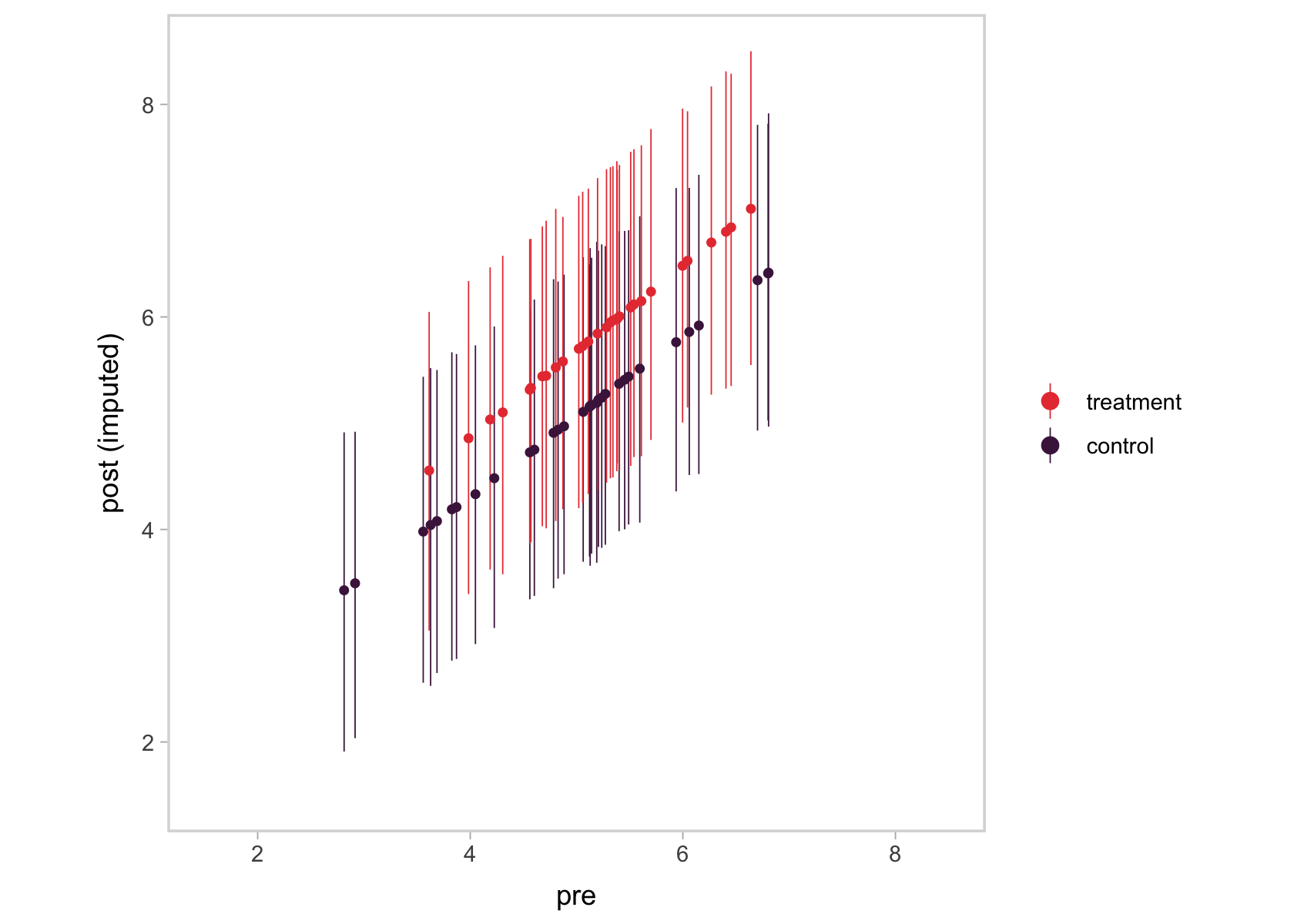
We ended up with something of a mash-up of a scatter plot and a coefficient plot. The \(y\)-axis shows the summaries for the imputed values, summarized by their posterior means (dots) and 95% intervals (vertical lines). In the \(x\)-axis, we’ve connected them with their original pre values. Notice the strong correlation between the two axes. That’s the consequence of fitting a bivariate model where pre has a residual correlation with post_observed. That original data-generating value, recall, was \(.75\). Here’s the summary of the residual correlation from fit2.

posterior_summary(fit2)["rescor__pre__postobserved", ] %>% 
  round(digits = 2)

##  Estimate Est.Error      Q2.5     Q97.5 
##      0.71      0.04      0.63      0.78

Using language perhaps more familiar to those from a structural equation modeling background, the pre values acted like a missing data covariate for the missing post_observed values. Had that residual correlation been lower, the relation in the two axes of our plot would have been less impressive, too. Anyway, the point is that one-step Bayesian imputation gives users a nice way to explore the missing data assumptions they’ve imposed in their models, which I think is pretty cool.

Would you like more?

To my knowledge, the introductory material on applied missing data analysis seems awash with full-information maximum likelihood and multiple imputation. One-step Bayesian imputation methods haven’t made it into the mainstream, yet. McElreath covered the one-step approach in both editions of his text and since the way he covered the material was quite different in the two editions, I really recommend you check out both ( McElreath, 2020, 2015). My ebook translations of McElreath’s texts covered that material from a brms + tidyverse perspective ( Kurz, 2021, 2020b). Otherwise, you should check out Bürkner’s ( 2021) vignette, Handle missing values with brms.

If you are aware of any other applied text books covering one-step Bayesian imputation, please drop a comment on this tweet.

New blog up!https://t.co/Drxd9jrdp1

This time we explore how to handle missing data in a 2-timepoint RCT with the one-step Bayesian imputation approach. It’s slick and simple and another reason to love #brms.

— Solomon Kurz (@SolomonKurz) July 28, 2021

Session info

sessionInfo()

## R version 4.2.0 (2022-04-22)
## Platform: x86_64-apple-darwin17.0 (64-bit)
## Running under: macOS Big Sur/Monterey 10.16
## 
## Matrix products: default
## BLAS:   /Library/Frameworks/R.framework/Versions/4.2/Resources/lib/libRblas.0.dylib
## LAPACK: /Library/Frameworks/R.framework/Versions/4.2/Resources/lib/libRlapack.dylib
## 
## locale:
## [1] en_US.UTF-8/en_US.UTF-8/en_US.UTF-8/C/en_US.UTF-8/en_US.UTF-8
## 
## attached base packages:
## [1] stats     graphics  grDevices utils     datasets  methods   base     
## 
## other attached packages:
##  [1] brms_2.18.0     Rcpp_1.0.9      tidybayes_3.0.2 faux_1.1.0      forcats_0.5.1   stringr_1.4.1   dplyr_1.0.10   
##  [8] purrr_0.3.4     readr_2.1.2     tidyr_1.2.1     tibble_3.1.8    ggplot2_3.4.0   tidyverse_1.3.2
## 
## loaded via a namespace (and not attached):
##   [1] readxl_1.4.1         backports_1.4.1      plyr_1.8.7           igraph_1.3.4         svUnit_1.0.6        
##   [6] splines_4.2.0        crosstalk_1.2.0      TH.data_1.1-1        rstantools_2.2.0     inline_0.3.19       
##  [11] digest_0.6.30        htmltools_0.5.3      fansi_1.0.3          magrittr_2.0.3       checkmate_2.1.0     
##  [16] googlesheets4_1.0.1  tzdb_0.3.0           modelr_0.1.8         RcppParallel_5.1.5   matrixStats_0.62.0  
##  [21] xts_0.12.1           sandwich_3.0-2       prettyunits_1.1.1    colorspace_2.0-3     rvest_1.0.2         
##  [26] ggdist_3.2.0         haven_2.5.1          xfun_0.35            callr_3.7.3          crayon_1.5.2        
##  [31] jsonlite_1.8.3       lme4_1.1-31          survival_3.4-0       zoo_1.8-10           glue_1.6.2          
##  [36] gtable_0.3.1         gargle_1.2.0         emmeans_1.8.0        distributional_0.3.1 pkgbuild_1.3.1      
##  [41] rstan_2.21.7         abind_1.4-5          scales_1.2.1         mvtnorm_1.1-3        DBI_1.1.3           
##  [46] miniUI_0.1.1.1       viridisLite_0.4.1    xtable_1.8-4         stats4_4.2.0         StanHeaders_2.21.0-7
##  [51] DT_0.24              htmlwidgets_1.5.4    httr_1.4.4           threejs_0.3.3        arrayhelpers_1.1-0  
##  [56] posterior_1.3.1      ellipsis_0.3.2       pkgconfig_2.0.3      loo_2.5.1            farver_2.1.1        
##  [61] sass_0.4.2           dbplyr_2.2.1         utf8_1.2.2           labeling_0.4.2       tidyselect_1.1.2    
##  [66] rlang_1.0.6          reshape2_1.4.4       later_1.3.0          munsell_0.5.0        cellranger_1.1.0    
##  [71] tools_4.2.0          cachem_1.0.6         cli_3.4.1            generics_0.1.3       broom_1.0.1         
##  [76] ggridges_0.5.3       evaluate_0.18        fastmap_1.1.0        yaml_2.3.5           processx_3.8.0      
##  [81] knitr_1.40           fs_1.5.2             nlme_3.1-159         mime_0.12            projpred_2.2.1      
##  [86] xml2_1.3.3           compiler_4.2.0       bayesplot_1.9.0      shinythemes_1.2.0    rstudioapi_0.13     
##  [91] gamm4_0.2-6          reprex_2.0.2         bslib_0.4.0          stringi_1.7.8        highr_0.9           
##  [96] ps_1.7.2             blogdown_1.15        Brobdingnag_1.2-8    lattice_0.20-45      Matrix_1.4-1        
## [101] nloptr_2.0.3         markdown_1.1         shinyjs_2.1.0        tensorA_0.36.2       vctrs_0.5.0         
## [106] pillar_1.8.1         lifecycle_1.0.3      jquerylib_0.1.4      bridgesampling_1.1-2 estimability_1.4.1  
## [111] httpuv_1.6.5         R6_2.5.1             bookdown_0.28        promises_1.2.0.1     gridExtra_2.3       
## [116] codetools_0.2-18     boot_1.3-28          colourpicker_1.1.1   MASS_7.3-58.1        gtools_3.9.3        
## [121] assertthat_0.2.1     withr_2.5.0          shinystan_2.6.0      multcomp_1.4-20      mgcv_1.8-40         
## [126] parallel_4.2.0       hms_1.1.1            grid_4.2.0           coda_0.19-4          minqa_1.2.5         
## [131] rmarkdown_2.16       googledrive_2.0.0    shiny_1.7.2          lubridate_1.8.0      base64enc_0.1-3     
## [136] dygraphs_1.1.1.6

References

Bürkner, P.-C. (2017). brms: An R package for Bayesian multilevel models using Stan. Journal of Statistical Software, 80(1), 1–28. https://doi.org/10.18637/jss.v080.i01
Bürkner, P.-C. (2018). Advanced Bayesian multilevel modeling with the R package brms. The R Journal, 10(1), 395–411. https://doi.org/10.32614/RJ-2018-017
Bürkner, P.-C. (2021). Handle missing values with brms. https://CRAN.R-project.org/package=brms/vignettes/brms_missings.html
Bürkner, P.-C. (2022). brms: Bayesian regression models using ’Stan’. https://CRAN.R-project.org/package=brms
Cohen, J. (1988). Statistical power analysis for the behavioral sciences. L. Erlbaum Associates. https://www.worldcat.org/title/statistical-power-analysis-for-the-behavioral-sciences/oclc/17877467
Cumming, G. (2012). Understanding the new statistics: Effect sizes, confidence intervals, and meta-analysis. Routledge. https://www.routledge.com/Understanding-The-New-Statistics-Effect-Sizes-Confidence-Intervals-and/Cumming/p/book/9780415879682
DeBruine, L. (2021). faux: Simulation for factorial designs [Manual]. https://github.com/debruine/faux
Enders, C. K. (2010). Applied missing data analysis. Guilford Press. http://www.appliedmissingdata.com/
Gelman, A., Hill, J., & Vehtari, A. (2020). Regression and other stories. Cambridge University Press. https://doi.org/10.1017/9781139161879
Kay, M. (2023). tidybayes: Tidy data and ’geoms’ for Bayesian models. https://CRAN.R-project.org/package=tidybayes
Kelley, K., & Preacher, K. J. (2012). On effect size. Psychological Methods, 17(2), 137. https://doi.org/10.1037/a0028086
Kruschke, J. K. (2015). Doing Bayesian data analysis: A tutorial with R, JAGS, and Stan. Academic Press. https://sites.google.com/site/doingbayesiandataanalysis/
Kurz, A. S. (2020a). Doing Bayesian data analysis in brms and the tidyverse (version 0.4.0). https://bookdown.org/content/3686/
Kurz, A. S. (2020b). Statistical rethinking with brms, ggplot2, and the tidyverse (version 1.2.0). https://doi.org/10.5281/zenodo.3693202
Kurz, A. S. (2021). Statistical rethinking with brms, ggplot2, and the tidyverse: Second Edition (version 0.2.0). https://bookdown.org/content/4857/
Little, R. J., & Rubin, D. B. (2019). Statistical analysis with missing data (3rd ed., Vol. 793). John Wiley & Sons. https://www.wiley.com/en-us/Statistical+Analysis+with+Missing+Data%2C+3rd+Edition-p-9780470526798
McElreath, R. (2015). Statistical rethinking: A Bayesian course with examples in R and Stan. CRC press. https://xcelab.net/rm/statistical-rethinking/
McElreath, R. (2020). Statistical rethinking: A Bayesian course with examples in R and Stan (Second Edition). CRC Press. https://xcelab.net/rm/statistical-rethinking/
R Core Team. (2022). R: A language and environment for statistical computing. R Foundation for Statistical Computing. https://www.R-project.org/
Walker, J. A. (2018). Elements of statistical modeling for experimental biology (“2020–11th–22” ed.). https://www.middleprofessor.com/files/applied-biostatistics_bookdown/_book/
Wickham, H. (2022). tidyverse: Easily install and load the ’tidyverse’. https://CRAN.R-project.org/package=tidyverse
Wickham, H., Averick, M., Bryan, J., Chang, W., McGowan, L. D., François, R., Grolemund, G., Hayes, A., Henry, L., Hester, J., Kuhn, M., Pedersen, T. L., Miller, E., Bache, S. M., Müller, K., Ooms, J., Robinson, D., Seidel, D. P., Spinu, V., … Yutani, H. (2019). Welcome to the tidyverse. Journal of Open Source Software, 4(43), 1686. https://doi.org/10.21105/joss.01686
-
As has been noted by others (e.g., McElreath, 2020) missing-data jargon is generally awful. I’m so sorry you have to contend with acronyms like MCAR, MAR (missing at random) and MNAR (missing not at random), but that’s just the way it is. If you’re not sure about the difference between the three, do consider spending some time with one of the missing data texts I recommended, above. ↩︎
- Posted on:
- July 27, 2021
- Length:
- 19 minute read, 3855 words