Regression models for 2-timepoint non-experimental data
By A. Solomon Kurz
December 29, 2020
Version 1.1.0
Edited on December 16, 2022, to use the new as_draws_df() workflow.
Purpose
In the contemporary longitudinal data analysis literature, 2-timepoint data (a.k.a. pre/post data) get a bad wrap. Singer and Willett ( 2003, p. 10) described 2-timepoint data as only “marginally better” than cross-sectional data and Rogosa et al. ( 1982) give a technical overview on the limitations of 2-timepoint data. Limitations aside, sometimes two timepoints are all you have. In those cases, researchers should have a good sense of which data analysis options they have at their disposal. I recently came across Jeffrey Walker’s free ( 2018) text, Elements of statistical modeling for experimental biology, which contains a nice chapter on 2-timepoint experimental designs. Inspired by his work, this post aims to explore how one might analyze non-experimental 2-timepoint data within a regression model paradigm.
I make assumptions.
In this post, I’m presuming you are familiar with longitudinal data analysis with conventional and multilevel regression. Though I don’t emphasize it much, it will also help if you’re familiar with Bayesian statistics. All code is in R ( R Core Team, 2022), with healthy doses of the tidyverse ( Wickham et al., 2019; Wickham, 2022). The statistical models will be fit with brms ( Bürkner, 2017, 2018, 2022) and we’ll also make some use of the tidybayes ( Kay, 2022) and patchwork ( Pedersen, 2022) packages. If you need to shore up, I list some educational resources at the end of the post.
Load the primary packages.
library(tidyverse)
library(brms)
library(tidybayes)
library(patchwork)
Warm-up
Before we jump into 2-timepoint data, we’ll first explore how one might analyze a fuller data set of 6 timepoints. We will then reduce the data set to two different 2-timepoint versions for use in the remainder of the post.
We need data.
We will simulate the data based on a conventional multilevel growth model of the kind you can learn about in Singer & Willett (
2003), Hoffman (
2015), or Kurz (
2020, Chapter 14). We’ll have one criterion variable \(y\) which will vary across participants \(i\) and over time \(t\). For simplicity, the systemic change over time will be linear. We might express it in statistical notation1 as
$$
\begin{align*} y_{ti} & \sim \operatorname{Normal}(\mu_{ti}, \sigma) \\ \mu_{ti} & = \beta_0 + \beta_1 \text{time}_{ti} + u_{0i} + u_{1i} \text{time}_{ti} \\ \sigma & = \sigma_\epsilon \\ \begin{bmatrix} u_{0i} \\ u_{1i} \end{bmatrix} & \sim \operatorname{MVNormal} \left (\begin{bmatrix} 0 \\ 0 \end{bmatrix}, \mathbf \Sigma \right) \\ \mathbf \Sigma & = \mathbf{SRS} \\ \mathbf S & = \begin{bmatrix} \sigma_0 & 0 \\ 0 & \sigma_1 \end{bmatrix} \\ \mathbf R & = \begin{bmatrix} 1 & \rho \\ \rho & 1 \end{bmatrix}, \end{align*}
$$
where \(\beta_0\) is the population-level intercept (initial status) and \(\beta_1\) is the population-level slope (change over time). The \(u_{0i}\) and \(u_{1i}\) terms are the participant-level deviations around the population-level intercept and slope. Those \(u\) deviations follow a bivariate normal distribution centered on zero (they are deviations, after all) and including a covariance matrix, \(\mathbf \Sigma\). As is typical within the brms framework (see
Bürkner, 2017), \(\mathbf \Sigma\) is decomposed into a matrix of standard deviations ($\mathbf S$) and a correlation matrix ($\mathbf R$). Also notice we renamed our original \(\sigma\) parameter as \(\sigma_\epsilon\) to help distinguish it from the multilevel standard deviations in the \(\mathbf S\) matrix ($\sigma_0$ and \(\sigma_1\)). In this way, \(\sigma_0\) and \(\sigma_1\) capture differences between participants in their intercepts and slopes, whereas \(\sigma_\epsilon\) captures the differences within participants over time that occur apart from their linear trajectories.
To simulate data of this kind, we’ll first set the true values for \(\beta_0, \beta_1, \sigma_0, \sigma_1, \rho,\) and \(\sigma_\epsilon\).
b0     <- 0      # starting point (average intercept)
b1     <- 1      # growth over time (average slope)
sigma0 <- 1      # std dev in intercepts
sigma1 <- 1      # std dev in slopes
rho    <- -.5    # correlation between intercepts and slopes
sigma_e <- 0.75  # std dev within participants
Now combine several of those values to define the \(\mathbf S, \mathbf R,\) and \(\mathbf \Sigma\) matrices. Then simulate \(N = 100\) participant-level intercepts and slopes.
mu     <- c(b0, b1)          # combine the means in a vector
sigmas <- c(sigma0, sigma1)  # combine the std devs in a vector

s <- diag(sigmas)      # standard deviation matrix
r <- matrix(c(1, rho,  # correlation matrix
             rho, 1), nrow = 2)

# now matrix multiply s and r to get a covariance matrix
sigma <- s %*% r %*% s

# how many participants would you like?
n_id <- 100

# make the simulation reproducible
set.seed(1)

vary_effects <-
  MASS::mvrnorm(n_id, mu = mu, Sigma = sigma) %>%
  data.frame() %>%
  set_names("intercepts", "slopes") %>%
  mutate(id = 1:n_id) %>%
  select(id, everything())

head(vary_effects)
##   id  intercepts     slopes
## 1  1  0.85270825  0.7676584
## 2  2 -0.18009772  1.1379818
## 3  3  1.17913643  0.7317852
## 4  4 -1.46056809  2.3025393
## 5  5  0.04193022  1.6126544
## 6  6 -0.17309717 -0.5941901
Now we have our random intercepts and slopes, we’re almost ready to simulate our \(y_{ti}\) values. We just need to decide on how many values we’d like to collect over time and how we’d like to structure those assessment periods. To keep things simple, I’m going to specify six evenly-spaced timepoints. The first timepoint will be set to 0, the last timepoint will be set to 1, and the four timepoints in the middle will be the corresponding fractions.
# how many timepoints?
time_points <- 6

d <-
  vary_effects %>%
  # add in time
  expand(nesting(id, intercepts, slopes),
         time = seq(from = 0, to = 1, length.out = time_points)) %>%
  # now use the model formula to compute y
  mutate(y = rnorm(n(), mean = intercepts + slopes * time, sd = sigma_e))

head(d, n = 10)
## # A tibble: 10 × 5
##       id intercepts slopes  time      y
##    <int>      <dbl>  <dbl> <dbl>  <dbl>
##  1     1      0.853  0.768   0    1.16
##  2     1      0.853  0.768   0.2  2.27
##  3     1      0.853  0.768   0.4  2.35
##  4     1      0.853  0.768   0.6  1.07
##  5     1      0.853  0.768   0.8 -0.247
##  6     1      0.853  0.768   1    3.49
##  7     2     -0.180  1.14    0    0.320
##  8     2     -0.180  1.14    0.2  0.453
##  9     2     -0.180  1.14    0.4  0.265
## 10     2     -0.180  1.14    0.6  0.885
Before we move on, I should acknowledge that this simulation workflow is heavily influenced by McElreath ( 2020, Chapter 14). You can find a similar workflow in the ( 2020) preprint by DeBruine and Barr, Understanding mixed effects models through data simulation.
Explore the data.
Before fitting the model, it might help if we look at what we’ve done. Here’s a scatter plot of the random intercepts and slopes.
# set the global plotting theme
theme_set(theme_linedraw() +
            theme(text = element_text(family = "Times"),
                  panel.grid = element_blank()))

p1 <-
  vary_effects %>%
  ggplot(aes(x = intercepts, y = slopes)) +
  geom_point() +
  stat_ellipse(color = "grey50")

p1
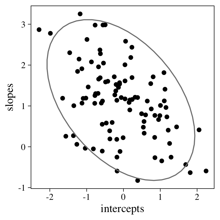
The 95%-interval ellipse helps point out the negative correlation between the intercepts and slopes. Here’s the Pearson’s correlation.
vary_effects %>%
  summarise(rho = cor(intercepts, slopes))
##          rho
## 1 -0.4502206
It’s no coincidence that value is very close to our data-generating rho value.
rho
## [1] -0.5
Now check the sample means and standard deviations of our intercepts and slopes.
vary_effects %>%
  summarise(b0 = mean(intercepts),
            b1 = mean(slopes),
            sigma0 = sd(intercepts),
            sigma1 = sd(slopes)) %>%
  mutate_all(round, digits = 2)
##      b0   b1 sigma0 sigma1
## 1 -0.08 1.11   0.91   0.91
Those aren’t quite the true data-generating values for b0 through sigma1, from above. But they’re pretty decent sample approximations. With only \(N = 100\) and \(T = 6\), this is about as close as we should expect.
To get a sense of the time and y values, we’ll plot them in two ways. First we’ll plot a random subset from nine of our simulated participants. Then we’ll plot the linear trajectories from all 100 participants, along with the grand mean trajectory.
set.seed(1)

p2 <-
  d %>%
  nest(data = c(intercepts, slopes, time, y)) %>%
  slice_sample(n = 9) %>%
  unnest(data) %>%

  ggplot(aes(x = time, y = y)) +
  geom_point() +
  geom_abline(aes(intercept = intercepts, slope = slopes),
              color = "blue") +
  labs(subtitle = "random subset of 9 participants") +
  theme(strip.background = element_blank(),
        strip.text = element_blank()) +
  facet_wrap(~slopes)

p3 <-
  d %>%
  ggplot(aes(x = time, y = y)) +
  geom_point(color = "transparent") +
  geom_abline(aes(intercept = intercepts, slope = slopes, group = id),
              color = "blue", linewidth = 1/10, alpha = 1/2) +
  geom_abline(intercept = b0, slope = b1,
              color = "blue", linewidth = 2) +
  labs(subtitle = "All participant-level trajectories, along\nwith the grand mean")

# combine
(p2 + p3) &
  scale_x_continuous(breaks = 0:5 / 5, labels = c(0, "", "", "", "", 1)) &
  coord_cartesian(ylim = c(-2.5, 3.5))
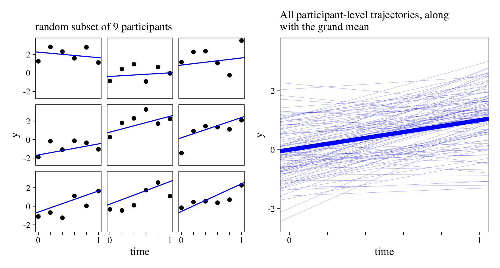
See how the points in the plots on the left deviate quite a bit from their linear trajectories? That’s the result of \(\sigma_\epsilon\).
Fit the multilevel growth model.
Now we’ll use brms to fit the multilevel growth model. If all goes well, we should largely reproduce our data-generating values in the posterior. Before fitting the model, we should consider a few things about the brm() syntax.
In this model and in most of the models to follow, we’re relying on the default brm() priors. When fitting real-world models, you are much better off going beyond the defaults. However, I will generally deemphasize priors, in this post, to help keep the focus on the conceptual models.
Note how we set the seed argument. Though you don’t need to do this, setting the seed makes the results more reproducible.
Also, note the custom settings for iter and warmup. Often times, the default settings are fine. But since we’ll be comparing a lot of models, I want to make sure we have enough posterior draws from each to ensure stable estimates.
Okay, fit the model.
m0 <-
  brm(data = d,
      y ~ 1 + time + (1 + time | id),
      seed = 1,
      cores = 4, chains = 4, iter = 3500, warmup = 1000)
Check the model summary.
print(m0)
##  Family: gaussian
##   Links: mu = identity; sigma = identity
## Formula: y ~ 1 + time + (1 + time | id)
##    Data: d (Number of observations: 600)
##   Draws: 4 chains, each with iter = 3500; warmup = 1000; thin = 1;
##          total post-warmup draws = 10000
##
## Group-Level Effects:
## ~id (Number of levels: 100)
##                     Estimate Est.Error l-95% CI u-95% CI Rhat Bulk_ESS Tail_ESS
## sd(Intercept)           0.89      0.09     0.72     1.08 1.00     3861     5490
## sd(time)                0.84      0.15     0.53     1.14 1.00     2269     3405
## cor(Intercept,time)    -0.40      0.15    -0.65    -0.07 1.00     4466     5670
##
## Population-Level Effects:
##           Estimate Est.Error l-95% CI u-95% CI Rhat Bulk_ESS Tail_ESS
## Intercept    -0.13      0.11    -0.35     0.08 1.00     4423     5692
## time          1.17      0.13     0.92     1.43 1.00     7499     7442
##
## Family Specific Parameters:
##       Estimate Est.Error l-95% CI u-95% CI Rhat Bulk_ESS Tail_ESS
## sigma     0.81      0.03     0.75     0.87 1.00     4880     6524
##
## Draws were sampled using sampling(NUTS). For each parameter, Bulk_ESS
## and Tail_ESS are effective sample size measures, and Rhat is the potential
## scale reduction factor on split chains (at convergence, Rhat = 1).
A series of plots might help show how well our model captured the data-generating values.
# name the parameters with the Greek terms
names <- c("beta[0]", "beta[1]", "sigma[0]", "sigma[1]", "rho", "sigma[epsilon]")

# for the vertical lines marking off the true values
vline <-
  tibble(name = names,
         true_value = c(b0, b1, sigma0, sigma1, rho, sigma_e))

# wrangle
as_draws_df(m0) %>%
  select(b_Intercept:sigma) %>%
  set_names(names) %>%
  pivot_longer(everything()) %>%

  # plot
  ggplot(aes(x = value, y = 0)) +
  stat_halfeye(.width = .95, normalize = "panels", size = 1/2) +
  geom_vline(data = vline,
             aes(xintercept = true_value),
             size = 1/4, linetype = 2) +
  scale_y_continuous(NULL, breaks = NULL) +
  xlab("marginal posterior") +
  facet_wrap(~name, scales = "free", labeller = label_parsed)
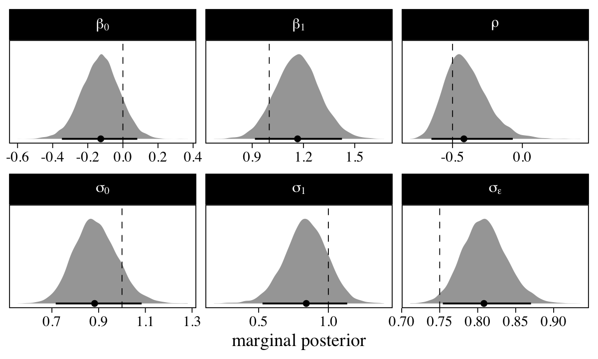
The marginal posterior distribution for all the major summary parameters is summarized by the median (dot) and percentile-based 95% interval (horizontal line). The true values are shown in the dashed vertical lines. Overall, we did okay.
As fun as this has all been, we’ve just been warming up.
Make the 2-timepoint data.
Before fitting the 2-timepoint longitudinal models, we’ll need to adjust the data, which currently contains values over six timepoints. Since it’s easy to think of 2-timepoint data in terms of pre and post, we’ll keep the data points for which time == 0 and time == 1.
small_data_long <-
  d %>%
  filter(time == 0 | time == 1) %>%
  select(-intercepts, -slopes) %>%
  mutate(`pre/post` = factor(if_else(time == 0, "pre", "post"),
                             levels = c("pre", "post")))

head(small_data_long)
## # A tibble: 6 × 4
##      id  time     y `pre/post`
##   <int> <dbl> <dbl> <fct>
## 1     1     0 1.16  pre
## 2     1     1 3.49  post
## 3     2     0 0.320 pre
## 4     2     1 1.27  post
## 5     3     0 0.879 pre
## 6     3     1 0.971 post
As the name implies, the small_data_long data are still in the long format. Hoffman (
2015) described this as the stacked format and Singer and Willett (
2003) called this a person-period data set. Each level of id has two rows, one for each level of time, which is an explicit variable. In this formulation, time == 0 is the same as the “pre” timepoint and time == 1 is the same as “post.” To help clarify that, we added a pre/post column.
We’ll need a second variant of this data set, this time in the wide format.
small_data_wide <-
  small_data_long %>%
  select(-time) %>%
  pivot_wider(names_from = `pre/post`, values_from = y) %>%
  mutate(change = post - pre)

head(small_data_wide)
## # A tibble: 6 × 4
##      id    pre   post change
##   <int>  <dbl>  <dbl>  <dbl>
## 1     1  1.16   3.49  2.33
## 2     2  0.320  1.27  0.953
## 3     3  0.879  0.971 0.0920
## 4     4 -0.979  0.586 1.57
## 5     5 -0.825  1.85  2.68
## 6     6 -0.912 -0.841 0.0715
With our small_data_wide data, each level of id only has one row. The time-structured y column was broken up into a pre and post column, and we no longer have a variable explicitly defining time. We have a new column, change, which is the result of subtracting pre from post. In her text, Hoffman referred to this type of data structure as the multivariate format and Singer and Willett called it a person-level data set.
The information is essentially the same in these two data sets, small_data_long and small_data_wide. Yet, the models supported by them will provide different insights.
2-timepoint longitudinal models
Before we start fitting and interpreting models, we should prepare ourselves with an overview.
Overview.
We will consider 20 ways to fit models based on 2-timepoint data. It seems like there multiple ways to categorize these. Here we’ll break them up into four groupings.
The first four model types will take post as the criterion:
\(\mathcal M_1 \colon\)The unconditional post model (post ~ 1),\(\mathcal M_2 \colon\)The simple autoregressive model (post ~ 1 + pre),\(\mathcal M_3 \colon\)The bivariate autoregressive model (bf(post ~ 1 + pre) + bf(pre ~ 1) + set_rescor(rescor = FALSE)), and\(\mathcal M_4 \colon\)The bivariate correlational pre/post model (bf(post ~ 1) + bf(pre ~ 1) + set_rescor(rescor = TRUE)).
The next four model types will take change as the criterion:
\(\mathcal M_5 \colon\)The unconditional change-score model (change ~ 1) and\(\mathcal M_6 \colon\)The conditional change-score model (change ~ 1 + pre).\(\mathcal M_7 \colon\)The bivariate conditional change-score model (bf(change ~ 1 + pre) + bf(pre ~ 1) + set_rescor(rescor = FALSE)), and\(\mathcal M_8 \colon\)The bivariate correlational pre/change model (bf(change ~ 1) + bf(pre ~ 1) + set_rescor(rescor = TRUE)).
The next eight model types will take y as the criterion:
\(\mathcal M_9 \colon\)The grand-mean model (y ~ 1),\(\mathcal M_{10} \colon\)The random-intercept model (y ~ 1 + (1 | id)),\(\mathcal M_{11} \colon\)The cross-classified model (y ~ 1 + (1 | id) + (1 | time)),\(\mathcal M_{12} \colon\)The simple liner model (y ~ 1 + time),\(\mathcal M_{13} \colon\)The liner model with a random intercept (y ~ 1 + time + (1 | id)),\(\mathcal M_{14} \colon\)The liner model with a random slope (y ~ 1 + time + (0 + time | id)),\(\mathcal M_{15} \colon\)The multilevel growth model with regularizing priors (y ~ 1 + time + (1 + time | id)), and\(\mathcal M_{16} \colon\)The fixed effects with correlated error model (y ~ 1 + time + ar(time = time, p = 1, gr = id).
The final four model types will expand previous ones with robust variance parameters:
\(\mathcal M_{17} \colon\)The cross-classified model with robust variances for discrete time (bf(y ~ 1 + (1 | id) + (1 | time), sigma ~ 0 + factor(time))),\(\mathcal M_{18} \colon\)The simple liner model with robust variance for linear time (bf(y ~ 1 + time, sigma ~ 1 + time)),\(\mathcal M_{19} \colon\)The liner model with correlated random intercepts for\(\mu\)and\(\sigma\)(bf(y ~ 1 + time + (1 |x| id), sigma ~ 1 + (1 |x| id))), and\(\mathcal M_{20} \colon\)The liner model with a random slope for\(\mu\)and uncorrelated random intercept for\(\sigma\)(bf(y ~ 1 + time + (0 + time | id), sigma ~ 1 + (1 | id))).
As far as these model names go, I’m making no claim they are canonical. Call them what you want. My goal, here, is to use names that are minimally descriptive and similar to the terms you might find used by other authors.
Models focusing on the second timepoint, post.
\(\mathcal M_1 \colon\) The unconditional post model.
We can write the unconditional post model as
$$
\begin{align*} \text{post}_i & \sim \operatorname{Normal}(\mu, \sigma) \\ \mu & = \beta_0, \end{align*}
$$
where \(\beta_0\) is both the model intercept and the estimate for the mean value of post. The focus this model places on post comes at the cost of any contextual information on what earlier values we might compare post to. Also, since the only variable in the model is post, this technically is not a 2-timepoint model. But given its connection to the models to follow, it’s worth working through.
Here’s how to fit the model with brms.
m1 <-
  brm(data = small_data_wide,
      post ~ 1,
      seed = 1,
      cores = 4, chains = 4, iter = 3500, warmup = 1000)
print(m1)
##  Family: gaussian
##   Links: mu = identity; sigma = identity
## Formula: post ~ 1
##    Data: small_data_wide (Number of observations: 100)
##   Draws: 4 chains, each with iter = 3500; warmup = 1000; thin = 1;
##          total post-warmup draws = 10000
##
## Population-Level Effects:
##           Estimate Est.Error l-95% CI u-95% CI Rhat Bulk_ESS Tail_ESS
## Intercept     1.02      0.12     0.79     1.25 1.00     7308     5232
##
## Family Specific Parameters:
##       Estimate Est.Error l-95% CI u-95% CI Rhat Bulk_ESS Tail_ESS
## sigma     1.18      0.09     1.03     1.36 1.00     7561     6026
##
## Draws were sampled using sampling(NUTS). For each parameter, Bulk_ESS
## and Tail_ESS are effective sample size measures, and Rhat is the potential
## scale reduction factor on split chains (at convergence, Rhat = 1).
We might compare those parameters with their sample values.
small_data_wide %>%
  summarise(mean = mean(post),
            sd = sd(post))
## # A tibble: 1 × 2
##    mean    sd
##   <dbl> <dbl>
## 1  1.02  1.16
If you only care about computing the population estimates for \(\mu_\text{post}\) and \(\sigma_\text{post}\), this model does a great job. With no other variables in the model, this approach does a poor job telling us about growth processes.
\(\mathcal M_2 \colon\) The simple autoregressive model.
The simple model with the pre scores predicting post is a substantial improvement from the previous one. It follows the form
$$
\begin{align*} \text{post}_i & \sim \operatorname{Normal}(\mu_i, \sigma) \\ \mu_i & = \beta_0 + \beta_1 \text{pre}_i, \end{align*}
$$
where the intercept \(\beta_0\) is the expected value of post when pre is at zero. As with many other regression contexts, centering the predictor pre at the mean or some other meaningful value can help make \(\beta_0\) more interpretable. Of greater interest is the \(\beta_1\) coefficient, which is the expected deviation from \(\beta_0\) for a one-unit increase in pre. But since pre and post are really the same variable y measured at two timepoints, it might be helpful if we express this model in another way. In perhaps more technical form, the simple model with pre predicting post is really an autoregressive model following the form
$$
\begin{align*} y_{ti} & \sim \operatorname{Normal}(\mu_i, \sigma) \\ \mu_i & = \beta_0 + \phi y_{t - 1,i}, \end{align*}
$$
where the criterion \(y\) varies across persons \(i\) and timepoints \(t\). Here we only have two timepoints, \(\text{post} = t\) and \(\text{pre} = t - 1\). The strength of association between \(y_t\) and \(y_{t - 1}\) captured by the autoregressive parameter \(\phi\), which is often expressed in a correlation metric.
Here’s how to fit the model with brm().
m2 <-
  brm(data = small_data_wide,
      post ~ 1 + pre,
      seed = 1,
      cores = 4, chains = 4, iter = 3500, warmup = 1000)
print(m2)
##  Family: gaussian
##   Links: mu = identity; sigma = identity
## Formula: post ~ 1 + pre
##    Data: small_data_wide (Number of observations: 100)
##   Draws: 4 chains, each with iter = 3500; warmup = 1000; thin = 1;
##          total post-warmup draws = 10000
##
## Population-Level Effects:
##           Estimate Est.Error l-95% CI u-95% CI Rhat Bulk_ESS Tail_ESS
## Intercept     1.05      0.12     0.83     1.28 1.00     7840     5840
## pre           0.24      0.10     0.04     0.44 1.00     8382     6508
##
## Family Specific Parameters:
##       Estimate Est.Error l-95% CI u-95% CI Rhat Bulk_ESS Tail_ESS
## sigma     1.15      0.08     1.00     1.33 1.00     9150     7004
##
## Draws were sampled using sampling(NUTS). For each parameter, Bulk_ESS
## and Tail_ESS are effective sample size measures, and Rhat is the potential
## scale reduction factor on split chains (at convergence, Rhat = 1).
Let’s compare the pre coefficient with the Pearson’s correlation between pre and post.
small_data_wide %>%
  summarise(correlation = cor(pre, post))
## # A tibble: 1 × 1
##   correlation
##         <dbl>
## 1       0.232
Well look at that. Recall that the \(\beta_0\) parameter is the expected value in post when the predictor pre is at zero. Though the sample mean for pre is very close to zero, it’s not exactly so.
small_data_wide %>%
  summarise(pre_mean = mean(pre))
## # A tibble: 1 × 1
##   pre_mean
##      <dbl>
## 1   -0.154
Here’s how to use that information to predict the mean value for post.
fixef(m2)[1, 1] + fixef(m2)[2, 1] * mean(small_data_wide$pre)
## [1] 1.016922
We can get a full posterior summary with aid from fitted().
nd <- tibble(pre = mean(small_data_wide$pre))

fitted(m2, newdata = nd)
##      Estimate Est.Error      Q2.5    Q97.5
## [1,] 1.016922 0.1142169 0.7981281 1.244375
\(\mathcal M_3 \colon\) The bivariate autoregressive model.
Though the simple autoregressive model gives us a sense of the strength of association between pre and post–and thus a sense of the stability in \(y\) over time–, it still lacks an explicit parameter for mean value of \(y\) at \(t - 1\). Enter the bivariate autoregressive model,
$$
\begin{align*} \text{post}_i & \sim \operatorname{Normal}(\mu_i, \sigma) \\ \text{pre}_i & \sim \operatorname{Normal}(\nu, \tau) \\ \mu_i & = \beta_0 + \beta_1 \text{pre}_i \\ \nu & = \gamma_0, \end{align*}
$$
where \(\text{post}_i\) is still modeled as a simple linear function of \(\text{pre}_i\), but now we also include an unconditional model for \(\text{pre}_i\). This will give us an explicit comparison for where we started at the outset ($\nu$) and where we ended up ($\mu_i$). We can fit this model using the brms multivariate syntax where the two submodels are encased in bf() statements (
Bürkner, 2021b). Also, be careful to use set_rescor(rescor = FALSE) to omit a residual correlation between the two. Their association is already handled with the \(\beta_1\) parameter.
m3 <-
  brm(data = small_data_wide,
      bf(post ~ 1 + pre) +
        bf(pre ~ 1) +
        set_rescor(rescor = FALSE),
      seed = 1,
      cores = 4, chains = 4, iter = 3500, warmup = 1000)
print(m3)
##  Family: MV(gaussian, gaussian)
##   Links: mu = identity; sigma = identity
##          mu = identity; sigma = identity
## Formula: post ~ 1 + pre
##          pre ~ 1
##    Data: small_data_wide (Number of observations: 100)
##   Draws: 4 chains, each with iter = 3500; warmup = 1000; thin = 1;
##          total post-warmup draws = 10000
##
## Population-Level Effects:
##                Estimate Est.Error l-95% CI u-95% CI Rhat Bulk_ESS Tail_ESS
## post_Intercept     1.05      0.12     0.83     1.28 1.00    12712     7848
## pre_Intercept     -0.15      0.12    -0.38     0.07 1.00    12373     7727
## post_pre           0.23      0.10     0.04     0.43 1.00    11614     7869
##
## Family Specific Parameters:
##            Estimate Est.Error l-95% CI u-95% CI Rhat Bulk_ESS Tail_ESS
## sigma_post     1.15      0.08     1.00     1.33 1.00    13103     8499
## sigma_pre      1.16      0.08     1.01     1.34 1.00    13596     7183
##
## Draws were sampled using sampling(NUTS). For each parameter, Bulk_ESS
## and Tail_ESS are effective sample size measures, and Rhat is the potential
## scale reduction factor on split chains (at convergence, Rhat = 1).
Now that we’ve broken out the multivariate syntax, we might consider a second bivariate model.
\(\mathcal M_4 \colon\) The bivariate correlational model.
The bivariate correlational model follows the form
$$
\begin{align*} \begin{bmatrix} \text{post}_i \\ \text{pre}_i \end{bmatrix} & \sim \operatorname{MVNormal} \left (\begin{bmatrix} \mu \\ \nu \end{bmatrix}, \mathbf \Sigma \right) \\ \mu & = \beta_0 \\ \nu & = \gamma_0 \\ \mathbf \Sigma & = \mathbf{SRS} \\ \mathbf S & = \begin{bmatrix} \sigma & 0 \\ 0 & \tau \end{bmatrix} \\ \mathbf R & = \begin{bmatrix} 1 & \rho \\ \rho & 1 \end{bmatrix}, \end{align*}
$$
where means of both pre and post are modeled in intercept-only models. However, the association between the two timepoints is captured in the residual correlation \(\rho\). Yet because we have no predictors in for either variable, the “residual” correlation is really just a correlation. We might also gain some insights if we re-express this model in terms of \(y_{ti}\) and \(y_{t - 1,i}\):
$$
\begin{align*} \begin{bmatrix} y_{ti} \\ y_{t - 1,i} \end{bmatrix} & \sim \operatorname{MVNormal} \left (\begin{bmatrix} \mu_t \\ \mu_{t - 1} \end{bmatrix}, \mathbf \Sigma \right) \\ \mu_t & = \beta_t \\ \mu_{t - 1} & = \beta_{t - 1} \\ \mathbf \Sigma & = \mathbf{SRS} \\ \mathbf S & = \begin{bmatrix} \sigma_t & 0 \\ 0 & \sigma_{t - 1} \end{bmatrix} \\ \mathbf R & = \begin{bmatrix} 1 & \rho \\ \rho & 1 \end{bmatrix}, \end{align*}
$$
where what we formerly called an autoregressive coefficient in \(\mathcal M_2\), we’re now calling a correlation. Note also that this model freely estimates \(\sigma_t\) and \(\sigma_{t - 1}\). In some contexts, these are presumed to be equal. Though we won’t be imposing that constraint, here, I believe it is possible with the brms
non-linear syntax (
Bürkner, 2021c). Anyway, here’s how to fit the model with the brm() function.
m4 <-
  brm(data = small_data_wide,
      bf(post ~ 1) +
        bf(pre ~ 1) +
        set_rescor(rescor = TRUE),
      seed = 1,
      cores = 4, chains = 4, iter = 3500, warmup = 1000)
Note out use of the set_rescor(rescor = TRUE) syntax in the model formula. This explicitly told brm() to include the residual correlation. Here’s the summary.
print(m4)
##  Family: MV(gaussian, gaussian)
##   Links: mu = identity; sigma = identity
##          mu = identity; sigma = identity
## Formula: post ~ 1
##          pre ~ 1
##    Data: small_data_wide (Number of observations: 100)
##   Draws: 4 chains, each with iter = 3500; warmup = 1000; thin = 1;
##          total post-warmup draws = 10000
##
## Population-Level Effects:
##                Estimate Est.Error l-95% CI u-95% CI Rhat Bulk_ESS Tail_ESS
## post_Intercept     1.02      0.12     0.78     1.25 1.00    10421     7309
## pre_Intercept     -0.15      0.11    -0.38     0.07 1.00    11377     8003
##
## Family Specific Parameters:
##            Estimate Est.Error l-95% CI u-95% CI Rhat Bulk_ESS Tail_ESS
## sigma_post     1.18      0.08     1.03     1.36 1.00    11641     8153
## sigma_pre      1.16      0.08     1.01     1.34 1.00    11444     7803
##
## Residual Correlations:
##                  Estimate Est.Error l-95% CI u-95% CI Rhat Bulk_ESS Tail_ESS
## rescor(post,pre)     0.23      0.09     0.03     0.40 1.00    11115     7824
##
## Draws were sampled using sampling(NUTS). For each parameter, Bulk_ESS
## and Tail_ESS are effective sample size measures, and Rhat is the potential
## scale reduction factor on split chains (at convergence, Rhat = 1).
Now the intercept and sigma parameters do a good job capturing the sample statistics.
small_data_wide %>%
  pivot_longer(pre:post) %>%
  group_by(name) %>%
  summarise(mean = mean(value),
            sd = sd(value)) %>%
  mutate_if(is.double, round, digits = 2)
## # A tibble: 2 × 3
##   name   mean    sd
##   <chr> <dbl> <dbl>
## 1 post   1.02  1.16
## 2 pre   -0.15  1.14
The new ‘rescor’ line at the bottom of the print() summary approximates the Pearson’s correlation of the two variables, much like the autoregressive parameter did two models up.
small_data_wide %>%
  summarise(correlation = cor(pre, post))
## # A tibble: 1 × 1
##   correlation
##         <dbl>
## 1       0.232
Another nice quality of this model is if you subtract \(\gamma_0\) from \(\beta_0\) (i.e., \(\beta_t - \beta_{t - 1}\)), you’d end up with the posterior mean of the change score.
as_draws_df(m4) %>%
  mutate(change = b_post_Intercept - b_pre_Intercept) %>%
  summarise(mu_change = mean(change))
## # A tibble: 1 × 1
##   mu_change
##       <dbl>
## 1      1.17
Keeping that in mind, let’s switch gears to the first of the change-score models.
Change-score models.
Instead of modeling post, \(y_{ti}\), we might instead want to focus on the change from pre to post, \(y_{ti} - y_{t - 1,i}\). When you subtract pre from post in your data set–like we did to make the change variable–, the product is often referred to as a change score or difference score, \(y_\Delta\). Though they’re conceptually intuitive and simple to compute, change scores have a long history of criticisms in the methodological literature, particularly around issues of reliability (see
Lord & Novick, 1968;
Rogosa et al., 1982; cf.
Kisbu-Sakarya et al., 2013). Here we consider four change-score models simply as options.
\(\mathcal M_5 \colon\) The unconditional change-score model.
We’ve already saved that in our small_data_wide data as change. Here’s what the unconditional change-score model2 looks like:
$$
\begin{align*} \text{change}_i & \sim \operatorname{Normal}(\mu, \sigma) \\ \mu & = \beta_0, \end{align*}
$$
where \(\beta_0\) is the expected value for \(\text{change}_i\). In the terms of the last model, \(\text{change}_i = \text{post}_i - \text{pre}_i\) or, in the terms of the simple autoregressive model, \(y_{\Delta i} = y_{ti} - y_{t - 1,i}\).
m5 <-
  brm(data = small_data_wide,
      change ~ 1,
      seed = 1,
      cores = 4, chains = 4, iter = 3500, warmup = 1000)
print(m5)
##  Family: gaussian
##   Links: mu = identity; sigma = identity
## Formula: change ~ 1
##    Data: small_data_wide (Number of observations: 100)
##   Draws: 4 chains, each with iter = 3500; warmup = 1000; thin = 1;
##          total post-warmup draws = 10000
##
## Population-Level Effects:
##           Estimate Est.Error l-95% CI u-95% CI Rhat Bulk_ESS Tail_ESS
## Intercept     1.17      0.15     0.88     1.45 1.00     8302     6607
##
## Family Specific Parameters:
##       Estimate Est.Error l-95% CI u-95% CI Rhat Bulk_ESS Tail_ESS
## sigma     1.45      0.10     1.26     1.66 1.00     8540     6890
##
## Draws were sampled using sampling(NUTS). For each parameter, Bulk_ESS
## and Tail_ESS are effective sample size measures, and Rhat is the potential
## scale reduction factor on split chains (at convergence, Rhat = 1).
Thus, this model suggests the average change from pre to post was about 1.2 units. We can compute the sample statistics for that in two ways.
small_data_wide %>%
  summarise(change = mean(change),
            `post - pre` = mean(post - pre))
## # A tibble: 1 × 2
##   change `post - pre`
##    <dbl>        <dbl>
## 1   1.17         1.17
The major deficit in the unconditional change model is that change is disconnected from any reference points. We have no explicit way of knowing what number we changed from or what number we changed to. The next model offers a solution.
\(\mathcal M_6 \colon\) The conditional change-score model.
Instead of fitting an unconditional model of change, why not condition on the initial pre value? We might express this as
$$
\begin{align*} \text{change}_i & \sim \operatorname{Normal}(\mu_i, \sigma) \\ \mu_i & = \beta_0 + \beta_1 \text{pre}_i, \end{align*}
$$
where \(\beta_0\) is now the expected value for change when pre is at zero. As with the simple autoregressive model, centering the predictor pre at the mean or some other meaningful value can help make \(\beta_0\) more interpretable. Perhaps of greater interest, the \(\beta_1\) coefficient allows us to predict different levels of change, conditional in the initial values at pre.
m6 <-
  brm(data = small_data_wide,
      change ~ 1 + pre,
      seed = 1,
      cores = 4, chains = 4, iter = 3500, warmup = 1000)
print(m6)
##  Family: gaussian
##   Links: mu = identity; sigma = identity
## Formula: change ~ 1 + pre
##    Data: small_data_wide (Number of observations: 100)
##   Draws: 4 chains, each with iter = 3500; warmup = 1000; thin = 1;
##          total post-warmup draws = 10000
##
## Population-Level Effects:
##           Estimate Est.Error l-95% CI u-95% CI Rhat Bulk_ESS Tail_ESS
## Intercept     1.05      0.12     0.82     1.28 1.00     9806     7007
## pre          -0.76      0.10    -0.97    -0.57 1.00     8867     7280
##
## Family Specific Parameters:
##       Estimate Est.Error l-95% CI u-95% CI Rhat Bulk_ESS Tail_ESS
## sigma     1.15      0.08     1.00     1.32 1.00     8128     6655
##
## Draws were sampled using sampling(NUTS). For each parameter, Bulk_ESS
## and Tail_ESS are effective sample size measures, and Rhat is the potential
## scale reduction factor on split chains (at convergence, Rhat = 1).
Since the intercept in this model is the expected change value based on when pre == 0, it might be easiest to interpret that value when using the mean of pre.
fixef(m6)[1, 1] + fixef(m6)[2, 1] * mean(small_data_wide$pre)
## [1] 1.16839
That is the point prediction for the mean of change. Let’s compare that to the sample value.
small_data_wide %>%
  summarise(mean = mean(change))
## # A tibble: 1 × 1
##    mean
##   <dbl>
## 1  1.17
Of course, we can get a fuller summary using the fitted() method.
nd <- tibble(pre = mean(small_data_wide$pre))

fitted(m6, newdata = nd)
##      Estimate Est.Error      Q2.5    Q97.5
## [1,]  1.16839  0.115271 0.9445871 1.395914
Note how the coefficient for pre is about -0.76. This is a rough analogue of the negative correlation among the intercepts and slopes in the original data-generating model.
rho
## [1] -0.5
It tells us something very similar; participants with higher values at pre tended to have lower change values. Much like with the simple autoregressive model, a deficit of this model is there is no explicit parameter for the expected value of pre, which we can amend by fitting a bivariate model.
\(\mathcal M_7 \colon\) The bivariate conditional change-score model.
The bivariate conditional change-score model follows the form
$$
\begin{align*} \text{change}_i & \sim \operatorname{Normal}(\mu_i, \sigma) \\ \text{pre}_i & \sim \operatorname{Normal}(\nu, \tau) \\ \mu_i & = \beta_0 + \beta_1 \text{pre}_i \\ \nu & = \gamma_0, \end{align*}
$$
where the simple linear model of \(\text{change}_i\) conditional on \(\text{pre}_i\) is coupled with an unconditional intercept-only model for \(\text{pre}_i\). We can fit this model with brms by way of the multivariate syntax, where the two submodels are encased in bf() statements and we set set_rescor(rescor = FALSE) to omit a residual correlation between the two.
m7 <-
  brm(data = small_data_wide,
      bf(change ~ 1 + pre) +
        bf(pre ~ 1) +
        set_rescor(rescor = FALSE),
      seed = 1,
      cores = 4, chains = 4, iter = 3500, warmup = 1000)
print(m7)
##  Family: MV(gaussian, gaussian)
##   Links: mu = identity; sigma = identity
##          mu = identity; sigma = identity
## Formula: change ~ 1 + pre
##          pre ~ 1
##    Data: small_data_wide (Number of observations: 100)
##   Draws: 4 chains, each with iter = 3500; warmup = 1000; thin = 1;
##          total post-warmup draws = 10000
##
## Population-Level Effects:
##                  Estimate Est.Error l-95% CI u-95% CI Rhat Bulk_ESS Tail_ESS
## change_Intercept     1.05      0.12     0.82     1.28 1.00    12639     7869
## pre_Intercept       -0.15      0.12    -0.38     0.08 1.00    11712     7316
## change_pre          -0.76      0.10    -0.96    -0.56 1.00    12822     6521
##
## Family Specific Parameters:
##              Estimate Est.Error l-95% CI u-95% CI Rhat Bulk_ESS Tail_ESS
## sigma_change     1.15      0.08     1.00     1.33 1.00    11945     8008
## sigma_pre        1.16      0.08     1.01     1.34 1.00    12657     7611
##
## Draws were sampled using sampling(NUTS). For each parameter, Bulk_ESS
## and Tail_ESS are effective sample size measures, and Rhat is the potential
## scale reduction factor on split chains (at convergence, Rhat = 1).
Now we have an intercept for pre, we can use the model parameters to compute the expected values for pre, change, and post.
as_draws_df(m7) %>%
  mutate(pre    = b_pre_Intercept,
         change = b_change_Intercept + b_change_pre * b_pre_Intercept) %>%
  mutate(post = pre + change) %>%
  pivot_longer(pre:post) %>%
  group_by(name) %>%
  mean_qi(value) %>%
  mutate_if(is.double, round, digits = 2)
## # A tibble: 3 × 7
##   name   value .lower .upper .width .point .interval
##   <chr>  <dbl>  <dbl>  <dbl>  <dbl> <chr>  <chr>
## 1 change  1.17   0.88   1.45   0.95 mean   qi
## 2 post    1.02   0.79   1.25   0.95 mean   qi
## 3 pre    -0.15  -0.38   0.08   0.95 mean   qi
The posterior means are in the value column and the lower- and upper-levels of the percentile-based 95% intervals are in the .lower and .upper columns. Now compare those mean estimates with the sample means.
small_data_wide %>%
  pivot_longer(-id) %>%
  group_by(name) %>%
  summarise(mean = mean(value)) %>%
  mutate_if(is.double, round, digits = 2)
## # A tibble: 3 × 2
##   name    mean
##   <chr>  <dbl>
## 1 change  1.17
## 2 post    1.02
## 3 pre    -0.15
As handy as this model is, the \(\beta_1\) coefficient might not be in the most intuitive metric. Let’s reparameterize.
\(\mathcal M_8 \colon\) The bivariate correlational pre/change model.
The bivariate correlational pre/change model follows the form
$$
\begin{align*} \begin{bmatrix} \text{change}_i \\ \text{pre}_i \end{bmatrix} & \sim \operatorname{MVNormal} \left (\begin{bmatrix} \mu \\ \nu \end{bmatrix}, \mathbf \Sigma \right) \\ \mu & = \beta_0 \\ \nu & = \gamma_0 \\ \mathbf \Sigma & = \mathbf{SRS} \\ \mathbf S & = \begin{bmatrix} \sigma & 0 \\ 0 & \tau \end{bmatrix} \\ \mathbf R & = \begin{bmatrix} 1 & \rho \\ \rho & 1 \end{bmatrix}, \end{align*}
$$
where means of both pre and change are modeled in intercept-only models and the association between the two is captured by the correlation \(\rho\). And again, because we have no predictors in for either variable, the “residual” correlation is really just a correlation. Here’s how to fit the model with brms.
m8 <-
  brm(data = small_data_wide,
      bf(change ~ 1) +
        bf(pre ~ 1) +
        set_rescor(rescor = TRUE),
      seed = 1,
      cores = 4, chains = 4, iter = 3500, warmup = 1000)
print(m8)
##  Family: MV(gaussian, gaussian)
##   Links: mu = identity; sigma = identity
##          mu = identity; sigma = identity
## Formula: change ~ 1
##          pre ~ 1
##    Data: small_data_wide (Number of observations: 100)
##   Draws: 4 chains, each with iter = 3500; warmup = 1000; thin = 1;
##          total post-warmup draws = 10000
##
## Population-Level Effects:
##                  Estimate Est.Error l-95% CI u-95% CI Rhat Bulk_ESS Tail_ESS
## change_Intercept     1.17      0.14     0.89     1.46 1.00     7847     7039
## pre_Intercept       -0.15      0.12    -0.39     0.07 1.00     8216     7486
##
## Family Specific Parameters:
##              Estimate Est.Error l-95% CI u-95% CI Rhat Bulk_ESS Tail_ESS
## sigma_change     1.45      0.10     1.26     1.67 1.00     8485     6858
## sigma_pre        1.16      0.08     1.01     1.33 1.00     9052     7486
##
## Residual Correlations:
##                    Estimate Est.Error l-95% CI u-95% CI Rhat Bulk_ESS Tail_ESS
## rescor(change,pre)    -0.60      0.06    -0.71    -0.47 1.00     8146     7142
##
## Draws were sampled using sampling(NUTS). For each parameter, Bulk_ESS
## and Tail_ESS are effective sample size measures, and Rhat is the potential
## scale reduction factor on split chains (at convergence, Rhat = 1).
Now the parameter in the ‘Residual Correlations’ section of the summary output is a close analogue to our original data-generating rho parameter.
rho
## [1] -0.5
Those with higher pre values tended to have lower change values. We can look at that with a plot of the data.
p2 <-
  small_data_wide %>%
  ggplot(aes(x = pre, y = change)) +
  geom_point() +
  stat_ellipse(color = "grey50")

(p1 + p2) &
  coord_cartesian(xlim = range(small_data_wide$pre),
                  ylim = range(small_data_wide$change))
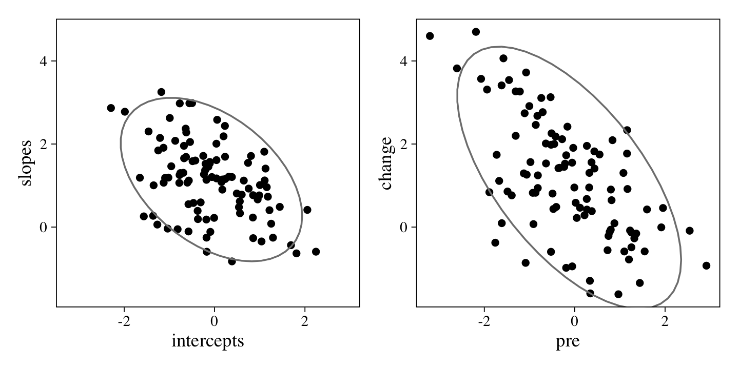
Here we’ve placed the scatter plot of the data-generating id-level intercepts and slopes next to the scatter plot of the pre and change scores. They are not exactly the same, but the latter are a partial consequence of the former. This is why the correlation parameter in our m8 model closely, but not exactly, resembled the data-generating rho parameter.
Okay, let’s switch gears again.
Models modeling the criterion \(y_{ti}\) directly.
All of the models focusing on post or change used the wide version of the data, small_data_wide. The remaining models will all take advantage of the long data set, small_data_long, and take \(y_{ti}\) as the criterion. Consequently, most of these models will use some version of the multilevel model.
\(\mathcal M_9 \colon\) The grand-mean model.
The simplest model we might fit using the long version of the 2-timepoint data, small_data_long, is what we might call the grand-mean model, or what Hoffman (
2015) called the between-person empty model. It follows the form
$$
\begin{align*} y_{ti} & \sim \operatorname{Normal}(\mu, \sigma) \\ \mu & = \beta_0, \end{align*}
$$
where the intercept \(\beta_0\) is the expected value value for \(y\) across all \(i\) participants and \(t\) timepoints. We fit this with brm() much like we fit the unconditional post model and the unconditional change-score model.
m9 <-
  brm(data = small_data_long,
      y ~ 1 ,
      seed = 1,
      cores = 4, chains = 4, iter = 3500, warmup = 1000)
print(m9)
##  Family: gaussian
##   Links: mu = identity; sigma = identity
## Formula: y ~ 1
##    Data: small_data_long (Number of observations: 200)
##   Draws: 4 chains, each with iter = 3500; warmup = 1000; thin = 1;
##          total post-warmup draws = 10000
##
## Population-Level Effects:
##           Estimate Est.Error l-95% CI u-95% CI Rhat Bulk_ESS Tail_ESS
## Intercept     0.43      0.09     0.25     0.61 1.00     7164     6291
##
## Family Specific Parameters:
##       Estimate Est.Error l-95% CI u-95% CI Rhat Bulk_ESS Tail_ESS
## sigma     1.30      0.07     1.18     1.43 1.00     8173     5821
##
## Draws were sampled using sampling(NUTS). For each parameter, Bulk_ESS
## and Tail_ESS are effective sample size measures, and Rhat is the potential
## scale reduction factor on split chains (at convergence, Rhat = 1).
We might check these with the sample statistics for y.
small_data_long %>%
  summarise(mean = mean(y),
            sd = sd(y))
## # A tibble: 1 × 2
##    mean    sd
##   <dbl> <dbl>
## 1 0.431  1.29
Though this model did to a good job describing the population values for the mean and standard deviation for y, it did a terrible job telling us about change in y, about individual differences in that change, or about anything else of interest we might have as longitudinal researchers.
\(\mathcal M_{10} \colon\) The random-intercept model.
Now that we have a grand mean, we might want to ask what kinds of variables would help explain the variation around the grand mean. From a multilevel perspective, the first source of variation of interest will be across participants, which we can express by allowing the mean to vary by participant. This is what Hoffman called the within-person empty model and the empty means, random intercept model. It follows the form
$$
\begin{align*} y_{ti} & \sim \operatorname{Normal}(\mu_i, \sigma) \\ \mu_i & = \beta_0 + u_{\text{id},i} \\ u_\text{id} & \sim \operatorname{Normal}(0, \sigma_\text{id}) \\ \sigma & = \sigma_\epsilon, \end{align*}
$$
where \(\beta_0\) is now the grand mean among the participant-level means in \(y_{ti}\). The participant-level deviations from the grand mean are expressed as \(u_{\text{id},i}\), which is normally distributed with a mean at zero (these are deviations, after all) and a standard deviation of \(\sigma_\text{id}\). The \(\sigma_\epsilon\) parameter is a mixture of the variation within participants and over time. With brms, we can fit the random-intercept model model like so.
m10 <-
  brm(data = small_data_long,
      y ~ 1 + (1 | id),
      seed = 1,
      cores = 4, chains = 4, iter = 3500, warmup = 1000,
      control = list(adapt_delta = .95))
print(m10)
##  Family: gaussian
##   Links: mu = identity; sigma = identity
## Formula: y ~ 1 + (1 | id)
##    Data: small_data_long (Number of observations: 200)
##   Draws: 4 chains, each with iter = 3500; warmup = 1000; thin = 1;
##          total post-warmup draws = 10000
##
## Group-Level Effects:
## ~id (Number of levels: 100)
##               Estimate Est.Error l-95% CI u-95% CI Rhat Bulk_ESS Tail_ESS
## sd(Intercept)     0.23      0.15     0.01     0.56 1.00     2533     3982
##
## Population-Level Effects:
##           Estimate Est.Error l-95% CI u-95% CI Rhat Bulk_ESS Tail_ESS
## Intercept     0.43      0.10     0.24     0.62 1.00    19133     7117
##
## Family Specific Parameters:
##       Estimate Est.Error l-95% CI u-95% CI Rhat Bulk_ESS Tail_ESS
## sigma     1.27      0.07     1.14     1.42 1.00     8106     6284
##
## Draws were sampled using sampling(NUTS). For each parameter, Bulk_ESS
## and Tail_ESS are effective sample size measures, and Rhat is the potential
## scale reduction factor on split chains (at convergence, Rhat = 1).
Our \(\beta_0\) intercept returned a very similar estimate for the grand mean, but we now interpret it as the grand mean for the within-person means for y. The variation in the id-level deviations around the grand mean, which we called \(u_{\text{id},i}\), is summarized by \(\sigma_\text{id}\) in the ‘Group-Level Effects’ section of the summary output.
Authors of many longitudinal text books (e.g., Hoffman, 2015; Singer & Willett, 2003) typically present this model as a way to directly compare the between- and within-person variation in the data by way of the intraclass correlation coefficient (ICC),
$$\text{ICC} = \frac{\text{between-person variance}}{\text{total variance}} = \frac{\sigma_\text{id}^2}{\sigma_\text{id}^2 + \sigma_\epsilon^2}.$$
When using frequentist methods, the ICC is typically expressed with a point estimate. When working with all our posterior draws, we can get full posterior distributions within the Bayesian framework.
as_draws_df(m10) %>%
  mutate(icc = sd_id__Intercept^2 / (sd_id__Intercept^2 + sigma^2)) %>%
  ggplot(aes(x = icc, y = 0)) +
  stat_halfeye(.width = .95) +
  scale_x_continuous("Intraclass correlation coefficient (ICC)",
                     breaks = 0:5 / 5, expand = c(0, 0), limits = 0:1) +
  scale_y_continuous(NULL, breaks = NULL)
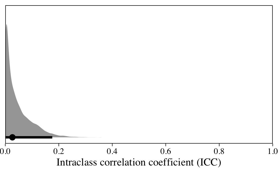
The ICC is a proportion, which limits it to the range of zero to one. Here it suggests that 0–20% of the variation in our data is due to differences between participants; the remaining variation occurs within them. Given that our data were collected across time, it might make sense to fit a model that explicitly accounts for time.
\(\mathcal M_{11} \colon\) The cross-classified model.
A direct extension of the random-intercept model is the cross-classified multilevel model ( McElreath, 2015, Chapter 12), which we might express as
$$
\begin{align*} y_{ti} & \sim \operatorname{Normal}(\mu_{ti}, \sigma) \\ \mu_{ti} & = \beta_0 + u_{\text{id},i} + u_{\text{time},i} \\ u_\text{id} & \sim \operatorname{Normal}(0, \sigma_\text{id}) \\ u_\text{time} & \sim \operatorname{Normal}(0, \sigma_\text{time}) \\ \sigma & = \sigma_\epsilon, \end{align*}
$$
where \(\sigma_\text{id}\) captures systemic differences between participants, \(\sigma_\text{time}\) captures systemic variation across the two timepoints, and \(\sigma_\epsilon\) captures the variation within participants over time. Another way to think of this model is as a Bayesian multilevel version of the repeated-measures ANOVA3, where variance is partitioned into a between level ($\sigma_\text{id} \approx \text{SS}\text{between}$), a model level ($\sigma\text{time} \approx \text{SS}\text{model}$), and error ($\sigma\epsilon \approx \text{SS}_\text{error}$).
m11 <-
  brm(data = small_data_long,
      y ~ 1 + (1 | time) + (1 | id),
      seed = 1,
      cores = 4, chains = 4, iter = 3500, warmup = 1000,
      control = list(adapt_delta = .999))
print(m11)
##  Family: gaussian
##   Links: mu = identity; sigma = identity
## Formula: y ~ 1 + (1 | time) + (1 | id)
##    Data: small_data_long (Number of observations: 200)
##   Draws: 4 chains, each with iter = 3500; warmup = 1000; thin = 1;
##          total post-warmup draws = 10000
##
## Group-Level Effects:
## ~id (Number of levels: 100)
##               Estimate Est.Error l-95% CI u-95% CI Rhat Bulk_ESS Tail_ESS
## sd(Intercept)     0.51      0.16     0.12     0.77 1.00     1618     1734
##
## ~time (Number of levels: 2)
##               Estimate Est.Error l-95% CI u-95% CI Rhat Bulk_ESS Tail_ESS
## sd(Intercept)     1.68      1.26     0.41     4.94 1.00     5779     6690
##
## Population-Level Effects:
##           Estimate Est.Error l-95% CI u-95% CI Rhat Bulk_ESS Tail_ESS
## Intercept     0.45      1.07    -1.74     2.77 1.00     4809     4823
##
## Family Specific Parameters:
##       Estimate Est.Error l-95% CI u-95% CI Rhat Bulk_ESS Tail_ESS
## sigma     1.04      0.08     0.90     1.20 1.00     2552     4559
##
## Draws were sampled using sampling(NUTS). For each parameter, Bulk_ESS
## and Tail_ESS are effective sample size measures, and Rhat is the potential
## scale reduction factor on split chains (at convergence, Rhat = 1).
The intercept is the grand mean across all measures of y. The first row in the ‘Group-Level Effects’ section is our summary for \(\sigma_\text{id}\), which gives us a sense of the variation between participants in their overall tendencies in the criterion y. If we use the as_draws_df(), we can even look at the posteriors for the \(u_{\text{id},i}\) parameters, themselves.
as_draws_df(m11) %>%
  pivot_longer(starts_with("r_id")) %>%

  ggplot(aes(x = value, y = reorder(name, value))) +
  stat_pointinterval(point_interval = mean_qi, .width = .95, size = 1/6) +
  scale_y_discrete(expression(italic(i)), breaks = NULL) +
  labs(subtitle = expression(sigma[id]~is~the~summary~of~the~variation~across~these),
       x = expression(italic(u)[id][','*italic(i)]))

Given that each of the \(u_{\text{id},i}\) parameters is based primarily on two data points (the two data points per participant), it should be no surprise they are fairly wide. Even a few more measurement occasions within participants will narrow them substantially. If you fit the same model using the original 6-timepoint data, you’ll see the 95% intervals are almost half as wide.
Perhaps of greater interest are the \(u_{\text{time},i}\) parameters. If you combine them with the intercept, you’ll get the model-based expected values at both timepoints.
as_draws_df(m11) %>%
  transmute(pre  = b_Intercept + `r_time[0,Intercept]`,
            post = b_Intercept + `r_time[1,Intercept]`) %>%
  pivot_longer(everything()) %>%
  group_by(name) %>%
  mean_qi(value) %>%
  mutate_if(is.double, round, digits = 2)
## # A tibble: 2 × 7
##   name  value .lower .upper .width .point .interval
##   <chr> <dbl>  <dbl>  <dbl>  <dbl> <chr>  <chr>
## 1 post   1.01   0.78   1.23   0.95 mean   qi
## 2 pre   -0.15  -0.38   0.08   0.95 mean   qi
The final variance parameter, \(\sigma_\text{time}\), captures the within-participant variation over time. With a model like this, it seems natural to directly compare the magnitudes of the three variance parameters, which answers the question: Where’s the variance at? Here we’ll do so with a plot.
as_draws_df(m11) %>%
  select(sd_id__Intercept:sigma) %>%
  set_names("sigma[id]", "sigma[time]", "sigma[epsilon]") %>%
  pivot_longer(everything()) %>%
  mutate(name = factor(name, levels = c("sigma[epsilon]", "sigma[time]", "sigma[id]"))) %>%

  ggplot(aes(x = value, y = name)) +
  stat_halfeye(.width = .95, size = 1, normalize = "xy") +
  scale_x_continuous("marginal posterior", expand = expansion(mult = c(0, 0.05)), breaks = c(0, 1, 2, 5)) +
  scale_y_discrete(NULL, labels = ggplot2:::parse_safe) +
  coord_cartesian(xlim = c(0, 5.25),
                  ylim = c(1.5, 3.5)) +
  theme(axis.text.y = element_text(hjust = 0))
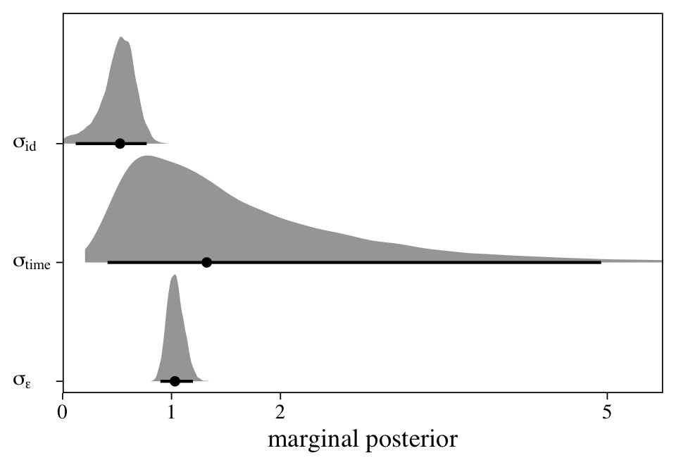
At first glance, it might be surprising how wide the \(\sigma_\text{time}\) posterior is compared to the other two. Yet recall this parameter is summarizing the standard deviation of only two levels. If you have experience with multilevel models, you’ll know that it can be difficult to estimate a variance parameter with few levels–two levels is the extreme lower limit. This is why we had to fiddle with the adapt_delta and max_treedepth parameters within the brm() function to get the model to sample properly. Though we pulled this off using default priors, don’t be surprised if you have to use tighter priors when fitting a model like this.
\(\mathcal M_{12} \colon\) The simple liner model.
The last three models focused on the grand mean and sources of variance around that grand mean. A more familiar looking approach might be to fit a simple linear model with y conditional on time,
$$
\begin{align*} y_{ti} & \sim \operatorname{Normal}(\mu_{ti}, \sigma) \\ \mu_{ti} & = \beta_0 + \beta_1 \text{time}_{ti}, \end{align*}
$$
where the intercept \(\beta_0\) is the expected value at the first timepoint and \(\beta_1\) captures the change in \(y_{ti}\) for the final timepoint.
m12 <-
  brm(data = small_data_long,
      y ~ 1 + time,
      seed = 1,
      cores = 4, chains = 4, iter = 3500, warmup = 1000)
print(m12)
##  Family: gaussian
##   Links: mu = identity; sigma = identity
## Formula: y ~ 1 + time
##    Data: small_data_long (Number of observations: 200)
##   Draws: 4 chains, each with iter = 3500; warmup = 1000; thin = 1;
##          total post-warmup draws = 10000
##
## Population-Level Effects:
##           Estimate Est.Error l-95% CI u-95% CI Rhat Bulk_ESS Tail_ESS
## Intercept    -0.16      0.11    -0.38     0.07 1.00     9236     6842
## time          1.17      0.16     0.86     1.48 1.00     9236     6973
##
## Family Specific Parameters:
##       Estimate Est.Error l-95% CI u-95% CI Rhat Bulk_ESS Tail_ESS
## sigma     1.16      0.06     1.05     1.28 1.00     8368     6768
##
## Draws were sampled using sampling(NUTS). For each parameter, Bulk_ESS
## and Tail_ESS are effective sample size measures, and Rhat is the potential
## scale reduction factor on split chains (at convergence, Rhat = 1).
Now our \(\beta_0\) and \(\beta_1\) parameters are the direct pre/post single-level analogues to the population-level \(\beta_0\) and \(\beta_1\) parameters from our original multilevel model based on the full 6-timepoint data set.
fixef(m0) %>% round(digits = 2)
##           Estimate Est.Error  Q2.5 Q97.5
## Intercept    -0.13      0.11 -0.35  0.08
## time          1.17      0.13  0.92  1.43
The major deficit in this model, which is the reason you’ll see it criticized in the methodological literature, is it ignores how the y values are nested within levels of id. The only variance parameter, \(\sigma\), was estimated under the typical assumption that the residuals are all independent of one another. Sure, the model formula accounted for the overall trend in time, but it ignored the insights revealed from many of the other models the capture between-participant correlations in intercepts and slopes. This means that if you know something about the value of one’s residual for when time == 0, you’ll also know something about where to expect their residual for when time == 1. The two are not independent. As long as we’re working with the data in the long format, we’ll want to account for this, somehow.
\(\mathcal M_{13} \colon\) The liner model with a random intercept.
A natural first step to accounting for how the y values are nested within levels of id is to fit a random-intercept model, or what Hoffman (
2015) called the fixed linear time, random intercept model. It follows the form
$$
\begin{align*} y_{ti} & \sim \operatorname{Normal}(\mu_{ti}, \sigma) \\ \mu_{ti} & = \beta_{0i} + \beta_1 \text{time}_{ti} \\ \beta_{0i} & = \gamma_0 + u_{0i} \\ u_{0i} & \sim \operatorname{Normal}(0, \sigma_0) \\ \sigma & = \sigma_\epsilon, \end{align*}
$$
where \(\beta_{0i}\) is the intercept and \(\beta_1\) is the time slope. Although this parameterization holds the variation in slopes constant across participants, between-participant variation is at least captured in \(\beta_{0i}\), which is decomposed into a grand mean, \(\gamma_0\), and participant-level deviations around that grand mean, \(u_{0i}\). Those participant-level deviations are summarized by the \(\sigma_0\) parameter. In this model, \(\sigma_\epsilon\) is a mixture of within-participant variation and between-participant variation in slopes.
m13 <-
  brm(data = small_data_long,
      y ~ 1 + time + (1 | id),
      seed = 1,
      cores = 4, chains = 4, iter = 3500, warmup = 1000)
print(m13)
##  Family: gaussian
##   Links: mu = identity; sigma = identity
## Formula: y ~ 1 + time + (1 | id)
##    Data: small_data_long (Number of observations: 200)
##   Draws: 4 chains, each with iter = 3500; warmup = 1000; thin = 1;
##          total post-warmup draws = 10000
##
## Group-Level Effects:
## ~id (Number of levels: 100)
##               Estimate Est.Error l-95% CI u-95% CI Rhat Bulk_ESS Tail_ESS
## sd(Intercept)     0.51      0.16     0.13     0.78 1.00     1455     1486
##
## Population-Level Effects:
##           Estimate Est.Error l-95% CI u-95% CI Rhat Bulk_ESS Tail_ESS
## Intercept    -0.15      0.11    -0.38     0.07 1.00    12585     8298
## time          1.17      0.15     0.88     1.46 1.00    18074     6862
##
## Family Specific Parameters:
##       Estimate Est.Error l-95% CI u-95% CI Rhat Bulk_ESS Tail_ESS
## sigma     1.03      0.08     0.89     1.19 1.00     2391     3976
##
## Draws were sampled using sampling(NUTS). For each parameter, Bulk_ESS
## and Tail_ESS are effective sample size measures, and Rhat is the potential
## scale reduction factor on split chains (at convergence, Rhat = 1).
The \(\beta\) parameters are very similar to those from the simple linear model, above.
fixef(m12) %>% round(digits = 2)
##           Estimate Est.Error  Q2.5 Q97.5
## Intercept    -0.16      0.11 -0.38  0.07
## time          1.17      0.16  0.86  1.48
But now look at the size of \(\sigma_0\), which suggests substantial differences in staring points. To get a sense of what this means, we’ll plot all 100 participant-level trajectories with a little help from fitted().
nd <- distinct(small_data_long, id, time)

fitted(m13,
       newdata = nd) %>%
  data.frame() %>%
  bind_cols(nd) %>%

  ggplot(aes(x = time, y = Estimate, group = id)) +
  geom_abline(intercept = fixef(m13)[1, 1],
              slope = fixef(m13)[2, 1],
              size = 3, color = "blue") +
  geom_line(size = 1/4, alpha = 2/3) +
  scale_x_continuous(breaks = 0:1) +
  labs(subtitle = "Random intercepts, fixed slope",
       y = "y") +
  coord_cartesian(ylim = c(-1, 2))
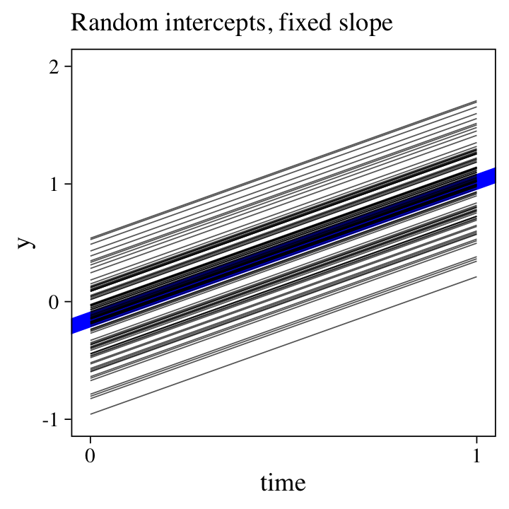
The bold blue line in the middle is based on the population-level intercept and slope, whereas the thinner black lines are the participant-level trajectories. To keep from overplotting, we’re only showing the posterior means, here. Because we only allowed the intercept to vary across participants, all the slopes are identical. And indeed, look at all the variation we see in the intercepts–an insight lacking in the simple linear model.
\(\mathcal M_{14} \colon\) The liner model with a random slope.
The counterpoint to the last model is to allow the time slopes, but not the intercepts, vary across participants:
$$
\begin{align*} y_{ti} & \sim \operatorname{Normal}(\mu_{ti}, \sigma) \\ \mu_{ti} & = \beta_0 + \beta_{1i} \text{time}_{ti} \\ \beta_{1i} & = \gamma_1 + u_{1i} \\ u_{1i} & \sim \operatorname{Normal}(0, \sigma_1) \\ \sigma & = \sigma_\epsilon, \end{align*}
$$
where \(\beta_0\) is the intercept for all participants. Now \(\beta_{1i}\) is the population mean for the distribution of slopes, which vary across participants, the standard deviation for which is measured by \(\sigma_1\).
m14 <-
  brm(data = small_data_long,
      y ~ 1 + time + (0 + time | id),
      seed = 1,
      cores = 4, chains = 4, iter = 3500, warmup = 1000,
      control = list(adapt_delta = .9))
print(m14)
##  Family: gaussian
##   Links: mu = identity; sigma = identity
## Formula: y ~ 1 + time + (0 + time | id)
##    Data: small_data_long (Number of observations: 200)
##   Draws: 4 chains, each with iter = 3500; warmup = 1000; thin = 1;
##          total post-warmup draws = 10000
##
## Group-Level Effects:
## ~id (Number of levels: 100)
##          Estimate Est.Error l-95% CI u-95% CI Rhat Bulk_ESS Tail_ESS
## sd(time)     0.32      0.20     0.02     0.74 1.00     1897     3410
##
## Population-Level Effects:
##           Estimate Est.Error l-95% CI u-95% CI Rhat Bulk_ESS Tail_ESS
## Intercept    -0.15      0.11    -0.37     0.07 1.00    15201     7635
## time          1.17      0.16     0.85     1.50 1.00    13510     6865
##
## Family Specific Parameters:
##       Estimate Est.Error l-95% CI u-95% CI Rhat Bulk_ESS Tail_ESS
## sigma     1.13      0.06     1.01     1.26 1.00     5591     4670
##
## Draws were sampled using sampling(NUTS). For each parameter, Bulk_ESS
## and Tail_ESS are effective sample size measures, and Rhat is the potential
## scale reduction factor on split chains (at convergence, Rhat = 1).
Here’s random-slopes alternative to the random-intercepts plot from the last section.
fitted(m14,
       newdata = nd) %>%
  data.frame() %>%
  bind_cols(nd) %>%

  ggplot(aes(x = time, y = Estimate, group = id)) +
  geom_abline(intercept = fixef(m14)[1, 1],
              slope = fixef(m14)[2, 1],
              size = 3, color = "blue") +
  geom_line(size = 1/4, alpha = 2/3) +
  scale_x_continuous(breaks = 0:1) +
  labs(subtitle = "Fixed intercept, random slopes",
       y = "y") +
  coord_cartesian(ylim = c(-1, 2))
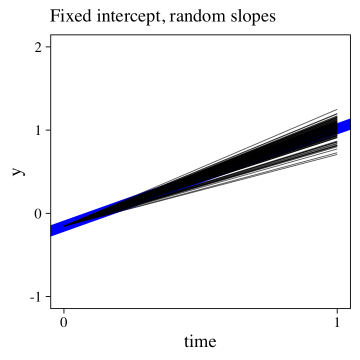
But why choose between random intercepts or random slopes?
\(\mathcal M_{15} \colon\) The multilevel growth model with regularizing priors.
If you were modeling 2-timepoint data with conventional frequentist estimators (e.g., maximum likelihood), you can have random intercepts or random slopes, but you can’t have both; that would require data from three timepoints or more. But because Bayesian models bring in extra information by way of the priors, you can actually fit a full multilevel growth model with both random intercepts and slopes:
$$
\begin{align*} y_{ti} & \sim \operatorname{Normal}(\mu_{ti}, \sigma_\epsilon ) \\ \mu_{ti} & = \beta_0 + \beta_1 \text{time}_{ti} + u_{0i} + u_{1i} \text{time}_{ti} \\ \begin{bmatrix} u_{0i} \\ u_{1i} \end{bmatrix} & \sim \operatorname{MVNormal} \left (\begin{bmatrix} 0 \\ 0 \end{bmatrix}, \mathbf \Sigma \right) \\ \mathbf \Sigma & = \mathbf{SRS} \\ \mathbf S & = \begin{bmatrix} \sigma_0 & 0 \\ 0 & \sigma_1 \end{bmatrix} \\ \mathbf R & = \begin{bmatrix} 1 & \rho \\ \rho & 1 \end{bmatrix}. \end{align*}
$$
The trick is you have to go beyond the diffuse brms default settings for the priors for \(\sigma_0\) and \(\sigma_1\). If you have high-quality information from theory or previous studies, you can base the priors on those. Another approach is to use regularizing priors. Given standardized data, members of the Stan team like either \(\operatorname{Normal}^+(0, 1)\) or \(\operatorname{Student-t}^+(3, 0, 1)\) for variance parameters (see the
Generic prior for anything section from the
Prior choice recommendations wiki). In the second edition of his text, McElreath generally favored the \(\operatorname{Exponential}(1)\) prior (
McElreath, 2020), which is the approach we’ll experiment with, here. It’ll also help if we use a regularizing prior on the correlation among the intercepts and slopes, \(\rho\).
m15 <-
  brm(data = small_data_long,
      y ~ 1 + time + (1 + time | id),
      seed = 1,
      prior = prior(exponential(1), class = sd) +
        prior(lkj(4), class = cor),
      cores = 4, chains = 4, iter = 3500, warmup = 1000,
      control = list(adapt_delta = .999))
Even with our tighter priors, we still had to adjust the adapt_delta parameter to improve the quality of the MCMC sampling. Take a look at the model summary.
print(m15)
##  Family: gaussian
##   Links: mu = identity; sigma = identity
## Formula: y ~ 1 + time + (1 + time | id)
##    Data: small_data_long (Number of observations: 200)
##   Draws: 4 chains, each with iter = 3500; warmup = 1000; thin = 1;
##          total post-warmup draws = 10000
##
## Group-Level Effects:
## ~id (Number of levels: 100)
##                     Estimate Est.Error l-95% CI u-95% CI Rhat Bulk_ESS Tail_ESS
## sd(Intercept)           0.50      0.18     0.08     0.82 1.01      860     1135
## sd(time)                0.30      0.23     0.01     0.85 1.00     1392     1082
## cor(Intercept,time)    -0.04      0.33    -0.63     0.62 1.00     5756     6702
##
## Population-Level Effects:
##           Estimate Est.Error l-95% CI u-95% CI Rhat Bulk_ESS Tail_ESS
## Intercept    -0.15      0.11    -0.37     0.07 1.00    13010     7120
## time          1.17      0.15     0.88     1.46 1.00    17027     7652
##
## Family Specific Parameters:
##       Estimate Est.Error l-95% CI u-95% CI Rhat Bulk_ESS Tail_ESS
## sigma     1.02      0.09     0.82     1.20 1.00      989     1062
##
## Draws were sampled using sampling(NUTS). For each parameter, Bulk_ESS
## and Tail_ESS are effective sample size measures, and Rhat is the potential
## scale reduction factor on split chains (at convergence, Rhat = 1).
Though the posteriors, particularly for the \(\sigma\) and \(\rho\) parameters, are not as precise as with the 6-timepoint data, we now have a model with a summary mirroring the structure of the data-generating model. Yet compared to the data-generating values, the estimates for \(\sigma_1\) and \(\rho\) are particularly biased toward zero. Here’s a look at the trajectories.
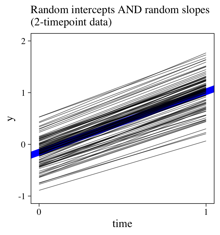
fitted(m15,
       newdata = nd) %>%
  data.frame() %>%
  bind_cols(nd) %>%

  ggplot(aes(x = time, y = Estimate, group = id)) +
  geom_abline(intercept = fixef(m15)[1, 1],
              slope = fixef(m15)[2, 1],
              size = 3, color = "blue") +
  geom_line(size = 1/4, alpha = 2/3) +
  scale_x_continuous(breaks = 0:1) +
  labs(subtitle = "Random intercepts AND random slopes\n(2-timepoint data)",
       y = "y") +
  coord_cartesian(ylim = c(-1, 2))
For comparision, here’s the plot for the original 6-timepoint model.
fitted(m0,
       newdata = nd) %>%
  data.frame() %>%
  bind_cols(nd) %>%

  ggplot(aes(x = time, y = Estimate, group = id)) +
  geom_abline(intercept = fixef(m0)[1, 1],
              slope = fixef(m0)[2, 1],
              size = 3, color = "blue") +
  geom_line(size = 1/4, alpha = 2/3) +
  scale_x_continuous(breaks = 0:1) +
  labs(subtitle = "Random intercepts AND random slopes\n(6-timepoint data)",
       y = "y") +
  coord_cartesian(ylim = c(-1, 2))
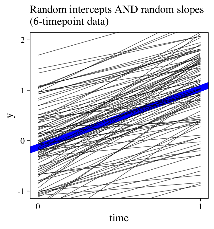
There wasn’t enough information in the 2-timepoint data set to capture the complexity in the full 6-timepoint data set.
\(\mathcal M_{16} \colon\) The fixed effects with correlated error model.
Though our Bayesian 2-timepoint version of the full multilevel growth model was exciting, it’s not generally used in the wild. Even with our tighter regularizing priors, there just wasn’t enough information in the data to do the model justice. A very different and humbler approach is to combine the simple linear model with the autoregressive model,
$$
\begin{align*} y_{ti} & \sim \operatorname{Normal}(\mu_{ti}, \mathbf \Sigma) \\ \mu_{ti} & = \beta_0 + \beta_1 \text{time}_{ti} \\ \mathbf \Sigma & = \mathbf{SRS} \\ \mathbf S & = \begin{bmatrix} \sigma & 0 \\ 0 & \sigma \end{bmatrix} \\ \mathbf R & = \begin{bmatrix} 1 & \rho \\ \rho & 1 \end{bmatrix}, \end{align*}
$$
where \(\rho\) captures the correlation between the responses in the two timepoints, \(t\) and \(t - 1\), which is an alternative to the way the mixed model from above handles the dependencies (a.k.a
heteroskedasticity) inherent in longitudinal data. Note how \(\mathbf \Sigma\) in this model is defined very differently from the full multilevel growth model from above. To fit this model with brms, we use the ar() syntax.
m16 <-
  brm(data = small_data_long,
      y ~ time + ar(time = time, p = 1, gr = id),
      seed = 1,
      cores = 4, chains = 4, iter = 3500, warmup = 1000)
print(m16)
##  Family: gaussian
##   Links: mu = identity; sigma = identity
## Formula: y ~ time + ar(time = time, p = 1, gr = id)
##    Data: small_data_long (Number of observations: 200)
##   Draws: 4 chains, each with iter = 3500; warmup = 1000; thin = 1;
##          total post-warmup draws = 10000
##
## Correlation Structures:
##       Estimate Est.Error l-95% CI u-95% CI Rhat Bulk_ESS Tail_ESS
## ar[1]     0.23      0.10     0.03     0.43 1.00     9988     7534
##
## Population-Level Effects:
##           Estimate Est.Error l-95% CI u-95% CI Rhat Bulk_ESS Tail_ESS
## Intercept    -0.15      0.11    -0.38     0.07 1.00    10585     7800
## time          1.17      0.14     0.89     1.45 1.00    10198     7749
##
## Family Specific Parameters:
##       Estimate Est.Error l-95% CI u-95% CI Rhat Bulk_ESS Tail_ESS
## sigma     1.15      0.06     1.04     1.27 1.00    11190     8254
##
## Draws were sampled using sampling(NUTS). For each parameter, Bulk_ESS
## and Tail_ESS are effective sample size measures, and Rhat is the potential
## scale reduction factor on split chains (at convergence, Rhat = 1).
This summary suggests that, after you account for the linear trend, the correlation between \(y_{ti}\) and \(y_{t - 1,i}\) is about 0.23. Though we don’t get id-specific variance parameters, this model does account for the nonindependence of the data over time. If you scroll back up, notice how similar this is to the correlation from the bivariate correlational model, m4.
The models with robust variance parameters.
In the social sciences, many of our theories and statistical models are comparisons of or changes in group means. Every model in this blog post uses the normal likelihood, which parameterizes the criterion in terms of \(\mu\) and \(\sigma\). Every time we added some kind of linear model, we focused that model around the \(\mu\). But contemporary Bayesian software allows us to model the \(\sigma\) parameter, too. Within the brms framework, Bürkner (
2021a) calls these
distributional models. The final four models under consideration all use some form of the distributional modeling syntax to relax unnecessarily restrictive assumptions on the variance parameters. Though this section is not exhaustive, it should give a sense of how flexible this approach can be.
\(\mathcal M_{17} \colon\) The cross-classified model with robust variances for discrete time.
One of the criticisms of the conventional repeated measures ANOVA approach is how it presumes the variances in \(y\) are constant over time. However, we can relax that constraint with a model like
$$
\begin{align*} y_{ti} & \sim \operatorname{Normal}(\mu_{ti}, \sigma_{ti}) \\ \mu_{ti} & = \beta_0 + u_{\text{id},i} + u_{\text{time},t} \\ \log (\sigma_{ti}) & = \eta_{\text{time},t} \\ u_\text{id} & \sim \operatorname{Normal}(0, \sigma_\text{id}) \\ u_\text{time} & \sim \operatorname{Normal}(0, \sigma_\text{time}), \end{align*}
$$
where we are now modeling both parameters in the likelihood, \(\mu\) AND \(\sigma\). The second line shows a typical-looking model for \(\mu_{ti}\). All the excitement lies in the third line, which contains the linear model for \(\log (\sigma_{ti})\). The reason we are modeling \(\log (\sigma_{ti})\) rather than directly modeling \(\sigma\) is to avoid solutions that predict negative values for \(\sigma\). For this model, it’s unlikely we’d run into that problem. But since the brms default is to use the log link anytime we model \(\sigma\) within the distributional modeling syntax, we’ll just get used to the log link right from the start. If you are unfamiliar with link functions, they’re widely used within the generalized linear modeling framework. Logistic regression with the logit link and Poisson regression with the log link are two widely-used examples. For more on link functions and the generalized linear model, check out the texts by Agresti (
2015); Gelman, Hill, and Vehtari (
2020); and McElreath (
2020,
2015).
Anyway, the linear model for \(\mu_{ti}\) is exactly the same as with the original cross-classified model, m11; it includes a grand mean ($\beta_0$) and two kinds of deviations around that grand mean ($u_{\text{id},i}$ and \(u_{\text{time},t}\)). The model for \(\log (\sigma_{ti})\) contains an intercept, which varies across the two levels of time, \(\eta_{\text{time},t}\). Here’s how to fit the model with brms::brm().
m17 <-
  brm(data = small_data_long,
      bf(y ~ 1 + (1 | time) + (1 | id),
         sigma ~ 0 + factor(time)),
      seed = 1,
      cores = 4, chains = 4, iter = 3500, warmup = 1000,
      control = list(adapt_delta = .995,
                     max_treedepth = 11))
print(m17)
##  Family: gaussian
##   Links: mu = identity; sigma = log
## Formula: y ~ 1 + (1 | time) + (1 | id)
##          sigma ~ 0 + factor(time)
##    Data: small_data_long (Number of observations: 200)
##   Draws: 4 chains, each with iter = 3500; warmup = 1000; thin = 1;
##          total post-warmup draws = 10000
##
## Group-Level Effects:
## ~id (Number of levels: 100)
##               Estimate Est.Error l-95% CI u-95% CI Rhat Bulk_ESS Tail_ESS
## sd(Intercept)     0.53      0.16     0.14     0.79 1.00     1333     1081
##
## ~time (Number of levels: 2)
##               Estimate Est.Error l-95% CI u-95% CI Rhat Bulk_ESS Tail_ESS
## sd(Intercept)     1.71      1.33     0.41     5.20 1.00     4622     6630
##
## Population-Level Effects:
##                   Estimate Est.Error l-95% CI u-95% CI Rhat Bulk_ESS Tail_ESS
## Intercept             0.45      1.11    -1.79     2.84 1.00     4656     4924
## sigma_factortime0     0.02      0.10    -0.19     0.21 1.00     3091     5239
## sigma_factortime1     0.03      0.10    -0.16     0.22 1.00     3324     5207
##
## Draws were sampled using sampling(NUTS). For each parameter, Bulk_ESS
## and Tail_ESS are effective sample size measures, and Rhat is the potential
## scale reduction factor on split chains (at convergence, Rhat = 1).
Even though we didn’t explicitly ask to use the log link in our brm() syntax, you can look at the second line in the print() output to see that it was automatically used. Though I won’t explore how to do so, here, one can fit this model without the log link. Anyway, the primary focus in this model is the sigma_factortime0 and sigma_factortime1 lines in the ‘Population-Level Effects’ section of the output. Those are the summaries for the \(\sigma\) parameters, conditional on whether time == 0 or time == 1. Though is might be difficult to evaluate parameters on the log scale, we can simply exponentiate them to convert them back to their natural metric.
fixef(m17)[2:3, c(1, 3:4)] %>% exp()
##                   Estimate      Q2.5    Q97.5
## sigma_factortime0 1.015122 0.8294728 1.235940
## sigma_factortime1 1.033489 0.8509822 1.251641
In this case, it looks like the two parameters are largely overlapping. If we work directly with the posterior draws, we can compute a formal difference score and plot the results.
as_draws_df(m17) %>%
  mutate(`sigma[time==0]` = exp(b_sigma_factortime0),
         `sigma[time==1]` = exp(b_sigma_factortime1),
         `sigma[time==1]-sigma[time==0]` = exp(b_sigma_factortime1) - exp(b_sigma_factortime0)) %>%
  pivot_longer(`sigma[time==0]`:`sigma[time==1]-sigma[time==0]`) %>%

  ggplot(aes(x = value, y = name)) +
  stat_halfeye(.width = .95) +
  scale_y_discrete(NULL, labels = ggplot2:::parse_safe,
                   expand = expansion(add = 0.1)) +
  xlab("marginal posterior") +
  theme(axis.text.y = element_text(hjust = 0))
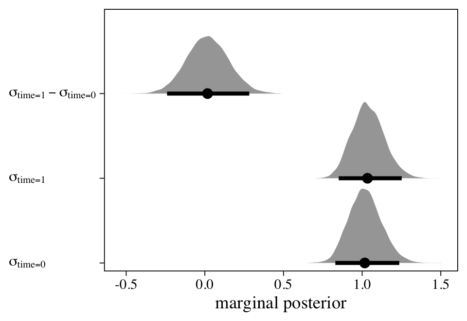
In this case, it looks like there was little difference between \(\sigma_{\text{time} = 0}\) and \(\sigma_{\text{time} = 1}\). This shouldn’t be a surprise; we simulated that data that way. However, it won’t always be like this in real-world data.
\(\mathcal M_{18} \colon\) The simple liner model with robust variance for linear time.
Our cross-classified approach treated time as a factor. Here we’ll treat it as a continuous variable in the models of both \(\mu\) and \(\sigma\). This will be a straight extension of the simple linear model, m12, following the form
$$
\begin{align*} y_{ti} & \sim \operatorname{Normal}(\mu_{ti}, \sigma_{ti}) \\ \mu_{ti} & = \beta_0 + \beta_1 \text{time}_{ti} \\ \log(\sigma_{ti}) & = \eta_0 + \eta_1 \text{time}_{ti}, \end{align*}
$$
where the intercept \(\beta_0\) is the expected value at the first timepoint and \(\beta_1\) captures the change in \(y_i\) for the final timepoint. Now \(\log(\sigma_{ti})\) has a similar linear model, where \(\eta_0\) is the expected log of the standard deviation at the first timepoint and \(\eta_1\) captures the change standard deviation for the final timepoint.
m18 <-
  brm(data = small_data_long,
      bf(y ~ 1 + time,
         sigma ~ 1 + time),
      seed = 1,
      cores = 4, chains = 4, iter = 3500, warmup = 1000)
print(m18)
##  Family: gaussian
##   Links: mu = identity; sigma = log
## Formula: y ~ 1 + time
##          sigma ~ 1 + time
##    Data: small_data_long (Number of observations: 200)
##   Draws: 4 chains, each with iter = 3500; warmup = 1000; thin = 1;
##          total post-warmup draws = 10000
##
## Population-Level Effects:
##                 Estimate Est.Error l-95% CI u-95% CI Rhat Bulk_ESS Tail_ESS
## Intercept          -0.16      0.12    -0.38     0.07 1.00    11435     8121
## sigma_Intercept     0.14      0.07     0.01     0.29 1.00    11081     7680
## time                1.17      0.16     0.84     1.49 1.00     9784     7464
## sigma_time          0.01      0.10    -0.19     0.21 1.00    11763     7839
##
## Draws were sampled using sampling(NUTS). For each parameter, Bulk_ESS
## and Tail_ESS are effective sample size measures, and Rhat is the potential
## scale reduction factor on split chains (at convergence, Rhat = 1).
Even though this model looks very different from the last one, we can wrangle the posterior draws a little to make a similar plot comparing \(\sigma\) at the two timepoints.
as_draws_df(m18) %>%
  mutate(`sigma[time==0]` = exp(b_sigma_Intercept),
         `sigma[time==1]` = exp(b_sigma_Intercept + b_sigma_time * 1),
         `sigma[time==1]-sigma[time==0]` = exp(b_sigma_Intercept) - exp(b_sigma_Intercept + b_sigma_time)) %>%
  pivot_longer(`sigma[time==0]`:`sigma[time==1]-sigma[time==0]`) %>%

  ggplot(aes(x = value, y = name)) +
  stat_halfeye(.width = .95) +
  scale_y_discrete(NULL, labels = ggplot2:::parse_safe,
                   expand = expansion(add = 0.1)) +
  xlab("marginal posterior") +
  theme(axis.text.y = element_text(hjust = 0))
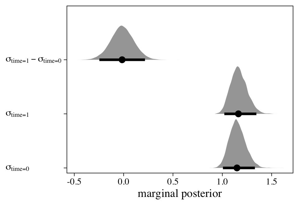
Though this model is robust to differences in \(\sigma\) based on timepoint, it still ignores systemic differences across participants. The next model tackles that that limitation in spades.
\(\mathcal M_{19} \colon\) The liner model with correlated random intercepts for \(\mu\) and \(\sigma.\)
Here we return to the multilevel model framework to accommodate participant-level differences for both \(\mu\) and \(\sigma\):
$$
\begin{align*} y_{ti} & \sim \operatorname{Normal}(\mu_{ti}, \sigma_{ti}) \\ \mu_{ti} & = \beta_0 + \beta_1 \text{time}_{ti} + u_{0i} \\ \log(\sigma_{ti}) & = \eta_0 + u_{2i} \\ \begin{bmatrix} u_{0i} \\ u_{2i} \end{bmatrix} & \sim \operatorname{MVNormal} \left (\begin{bmatrix} 0 \\ 0 \end{bmatrix}, \mathbf \Sigma \right) \\ \mathbf \Sigma & = \mathbf{SRS} \\ \mathbf S & = \begin{bmatrix} \sigma_0 & 0 \\ 0 & \sigma_2 \end{bmatrix} \\ \mathbf R & = \begin{bmatrix} 1 & \rho \\ \rho & 1 \end{bmatrix}, \end{align*}
$$
where \(\beta_0\) is the grand mean for the intercepts and \(u_{0i}\) are the participant-level deviations around that grand mean. \(\beta_1\) is the time slope, which is invariant across all participants in this model. The \(\eta_0\) parameter is the grand mean for the log standard deviations and \(u_{2i}\) captures the participant-level deviations around that grand mean. In the fourth line, we learn that \(u_{0i}\) and \(u_{2i}\) are multivariate normal, with a mean vector of two zeros and a variance/covariance matrix \(\mathbf \Sigma\). As is typical within the brms framework, we decompose \(\mathbf \Sigma\) into a variance matrix \(\mathbf S\) and correlation matrix \(\mathbf R\). Of particular interest is the \(\rho\) parameter, which captures the correlation in the participant-level intercepts and participant-level standard deviations. Here’s how to fit the model with brms.
m19 <-
  brm(data = small_data_long,
      bf(y ~ 1 + time + (1 |x| id),
         sigma ~ 1 + (1 |x| id)),
      seed = 1,
      cores = 4, chains = 4, iter = 3500, warmup = 1000,
      control = list(adapt_delta = .85))
You may have noticed the |x| parts in the formula lines for y and sigma. What that did was tell brms we wanted those parameters to be correlated. That is, that’s how we estimated the \(\rho\) parameter. There was nothing special about including x between the vertical lines. We could have used any other character. The important thing is that we used the same character in both. Anyway, here’s the model summary.
print(m19)
##  Family: gaussian
##   Links: mu = identity; sigma = log
## Formula: y ~ 1 + time + (1 | x | id)
##          sigma ~ 1 + (1 | x | id)
##    Data: small_data_long (Number of observations: 200)
##   Draws: 4 chains, each with iter = 3500; warmup = 1000; thin = 1;
##          total post-warmup draws = 10000
##
## Group-Level Effects:
## ~id (Number of levels: 100)
##                                Estimate Est.Error l-95% CI u-95% CI Rhat Bulk_ESS Tail_ESS
## sd(Intercept)                      0.52      0.16     0.12     0.78 1.00     1441     1593
## sd(sigma_Intercept)                0.11      0.08     0.01     0.29 1.00     3229     5582
## cor(Intercept,sigma_Intercept)    -0.34      0.49    -0.97     0.82 1.00     7197     5732
##
## Population-Level Effects:
##                 Estimate Est.Error l-95% CI u-95% CI Rhat Bulk_ESS Tail_ESS
## Intercept          -0.15      0.12    -0.38     0.08 1.00    11738     8198
## sigma_Intercept     0.01      0.08    -0.13     0.17 1.00     2465     4093
## time                1.17      0.15     0.88     1.46 1.00    15872     7611
##
## Draws were sampled using sampling(NUTS). For each parameter, Bulk_ESS
## and Tail_ESS are effective sample size measures, and Rhat is the potential
## scale reduction factor on split chains (at convergence, Rhat = 1).
Once again, brms used the log link for \(\sigma\). If you want to see \(\eta_0\) in its natural \(\sigma\) metric, exponentiate.
fixef(m19)["sigma_Intercept", c(1, 3:4)] %>% exp()
##  Estimate      Q2.5     Q97.5
## 1.0147602 0.8756565 1.1870699
The sd(sigma_Intercept) row in the ‘Group-Level Effects’ section shows the variation in those \(\log \sigma\)’s. It might be easier to appreciate them in a plot.
as_draws_df(m19) %>%
  pivot_longer(starts_with("r_id__sigma")) %>%
  mutate(sigma_i = exp(sd_id__sigma_Intercept + value)) %>%

  ggplot(aes(x = sigma_i, y = reorder(name, sigma_i))) +
  stat_pointinterval(point_interval = mean_qi, .width = .95, size = 1/6) +
  scale_y_discrete(expression(italic(i)), breaks = NULL) +
  labs(subtitle = expression(sigma[2]~summarizes~the~variation~across~these),
       x = expression(sigma[italic(i)]))
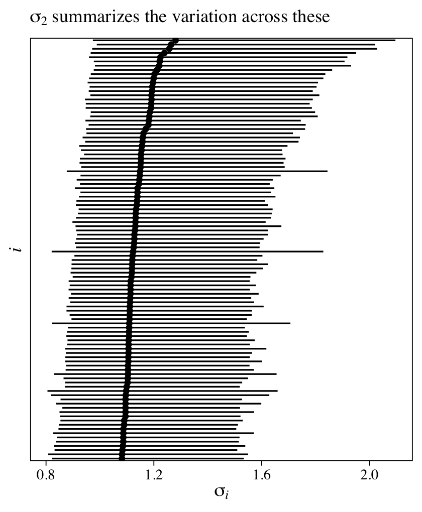
In this case, there was not a lot of variation in \(\sigma\) across participants. This is because we simulated the data that way. Though it may be hard to model participant-level variances with 2-timepoint data, I have found it comes in handy in real-world data sets based on more measurement occasions.
Finally, it might be useful to consider our \(\rho\) parameter, which suggested a mild negative correlation between the \(u_{0i}\) and \(u_{2i}\) deviations. Here’s how you might visualize that in a plot.
bind_rows(
  as_draws_df(m19) %>% select(starts_with("r_id[")) %>% set_names(1:100),
  as_draws_df(m19) %>% select(starts_with("r_id__sigma") %>% set_names(1:100))
) %>%
  mutate(iter = rep(1:c(n() / 2), times = 2),
         type = rep(c("intercept", "log_sigma"), each = n() / 2)) %>%
  pivot_longer(-c(iter, type)) %>%
  pivot_wider(names_from = type, values_from = value) %>%

  ggplot(aes(x = intercept, y = log_sigma, group = name)) +
  stat_ellipse(geom = "polygon", level = .01, alpha = 1/4) +
  labs(x = expression(italic(u)[0][italic(i)]),
       y = expression(log(italic(u)[2][italic(i)])))
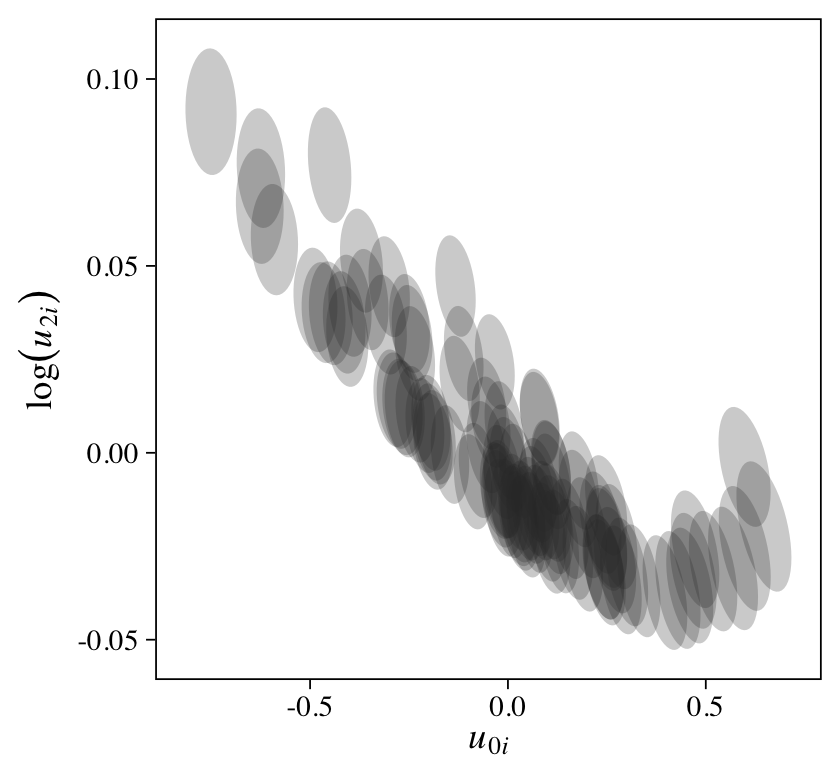
Each of the ovals is a 1% ellipse of the bivariate posterior for \(u_{0i}\) and \(\log(u_{2i})\). Notice how using ellipses helps reveal the differences in the between- and within-person patterns.
This approach where residual variance parameters vary across participants has its origins in the work of Donald Hedeker and colleagues ( Hedeker et al., 2008, 2012). More recently, Philippe Rast and colleagues (particularly graduate student, Donald Williams) have adapted this approach for use within the Stan/brms ecosystem ( Williams, Liu, et al., 2019; Williams, Rouder, et al., 2019; Williams, Martin, et al., 2019; Williams, Zimprich, et al., 2019).
\(\mathcal M_{20} \colon\) The liner model with a random slope for \(\mu\) and uncorrelated random intercept for \(\sigma\).
Though we can find interesting things when we allow the random components in the \(\mu\) and \(\sigma\) models, we don’t have to think of them as covarying. Here we fit an extension of the linear model with a random time slope, where we add an orthogonal random intercept for \(\sigma\):
$$
\begin{align*} y_{ti} & \sim \operatorname{Normal}(\mu_{ti}, \sigma_{ti}) \\ \mu_{ti} & = \beta_0 + \beta_1 \text{time}_{ti} + u_{1i} \\ \log(\sigma_{ti}) & = \eta_0 + u_{2i} \\ u_{1i} & \sim \operatorname{Normal}(0, \sigma_1) \\ u_{2i} & \sim \operatorname{Normal}(0, \sigma_2), \end{align*}
$$
where the two random components, \(u_{1i}\) and \(u_{2i}\), are now modeled with separate normal distributions, \(\operatorname{Normal}(0, \sigma_1)\) and \(\operatorname{Normal}(0, \sigma_2)\).
m20 <-
  brm(data = small_data_long,
      bf(y ~ 1 + time + (0 + time | id),
         sigma ~ 1 + (1 | id)),
      seed = 1,
      cores = 4, chains = 4, iter = 3500, warmup = 1000,
      control = list(adapt_delta = .85))
Note that in sharp contrast with our syntax for the previous model, this time we did not employ the |x| syntax in the formula lines for y and sigma. By omitting the |x| syntax, we omitted the correlation among those two random effects. Here’s the summary.
print(m20)
##  Family: gaussian
##   Links: mu = identity; sigma = log
## Formula: y ~ 1 + time + (0 + time | id)
##          sigma ~ 1 + (1 | id)
##    Data: small_data_long (Number of observations: 200)
##   Draws: 4 chains, each with iter = 3500; warmup = 1000; thin = 1;
##          total post-warmup draws = 10000
##
## Group-Level Effects:
## ~id (Number of levels: 100)
##                     Estimate Est.Error l-95% CI u-95% CI Rhat Bulk_ESS Tail_ESS
## sd(time)                0.33      0.21     0.01     0.76 1.00     2035     3722
## sd(sigma_Intercept)     0.12      0.08     0.01     0.31 1.00     3042     5110
##
## Population-Level Effects:
##                 Estimate Est.Error l-95% CI u-95% CI Rhat Bulk_ESS Tail_ESS
## Intercept          -0.15      0.11    -0.37     0.07 1.00    19053     7475
## sigma_Intercept     0.11      0.06    -0.03     0.22 1.00     5798     6327
## time                1.18      0.16     0.86     1.50 1.00    18653     7625
##
## Draws were sampled using sampling(NUTS). For each parameter, Bulk_ESS
## and Tail_ESS are effective sample size measures, and Rhat is the potential
## scale reduction factor on split chains (at convergence, Rhat = 1).
We can see the \(\sigma_1\) and \(\sigma_2\) summaries in the ‘Group-Level Effects’ section. It’s hard to compare them directly, because one is based on parameters in the log metric. But we can at least get a sense of what these parameters are summarizing by plotting the bivariate posterior for \(u_{1i}\) and \(\log(u_{2i})\).
bind_rows(
  as_draws_df(m20) %>% select(starts_with("r_id[")) %>% set_names(1:100),
  as_draws_df(m20) %>% select(starts_with("r_id__sigma") %>% set_names(1:100))
) %>%
  mutate(iter = rep(1:c(n() / 2), times = 2),
         type = rep(c("slope", "log_sigma"), each = n() / 2)) %>%
  pivot_longer(-c(iter, type)) %>%
  pivot_wider(names_from = type, values_from = value) %>%

  ggplot(aes(x = slope, y = log_sigma, group = name)) +
  stat_ellipse(geom = "polygon", level = .01, alpha = 1/4) +
  labs(x = expression(italic(u)[1][italic(i)]),
       y = expression(log(italic(u)[2][italic(i)])))
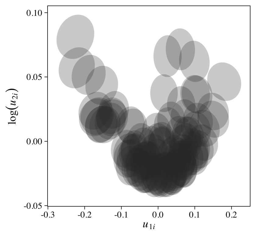
Notice how, this time, the 1% ellipses suggest no clear association between these two dimensions.
Next steps
As promised, here I recommend some resources for understanding the models in this post.
Books focusing on longutidinal data analysis.
-
My introduction to longitudinal data analysis was through Singer and Willett ( 2003), Applied longitudinal data analysis: Modeling change and event occurrence. Their focus was on the multilevel growth model and on survival analysis, primary from a maximum-likelihood frequentist framework. However, they generally avoided 2-timepoint data analysis.
-
Hoffman’s ( 2015) text, Longitudinal analysis: Modeling within-person fluctuation and change is another thorough introduction to the multilevel growth model, from a frequentist perspective. Hoffman covered 2-timepoint data analysis and variants from the ANOVA family. The text comes with a companion website, https://www.pilesofvariance.com/, which contains extensive data and code files for reproducing the material.
-
Newsom’s ( 2015) text, Longitudinal structural equation modeling: A comprehensive introduction, covers longitudinal data analysis from a structural equation modeling (SEM) perspective. Even for those not interested in SEM, his Chapter 4 does a nice job introducing the autoregressive and change-score models. The companion website, http://www.longitudinalsem.com/, contains data and script files for most of the problems in the text.
Books introducing regression.
-
Gelman, Hill, and Vehtari’s ( 2020) Regression and other stories contains a thorough introduction to single-level regression, primarily from a Bayesian framework. The text is not oriented around longitudinal analyses, per se, but it does include several chapters on causal inference. Vehtari hosts a GitHub repo, https://github.com/avehtari/ROS-Examples, where you can download the data files and R scripts for many of the examples.
-
Both editions of McElreath’s ( 2020, 2015) Statistical rethinking: A Bayesian course with examples in R and Stan provide a thorough introduction to Bayesian regression, both single-level and multilevel. McElreath also touched on causal inference and included a few examples of longitudinal data analysis. His text includes extensive examples of R code and his website, https://xcelab.net/rm/statistical-rethinking/, contains information about the accompanying statistical software.
Session info
sessionInfo()
## R version 4.2.0 (2022-04-22)
## Platform: x86_64-apple-darwin17.0 (64-bit)
## Running under: macOS Big Sur/Monterey 10.16
##
## Matrix products: default
## BLAS:   /Library/Frameworks/R.framework/Versions/4.2/Resources/lib/libRblas.0.dylib
## LAPACK: /Library/Frameworks/R.framework/Versions/4.2/Resources/lib/libRlapack.dylib
##
## locale:
## [1] en_US.UTF-8/en_US.UTF-8/en_US.UTF-8/C/en_US.UTF-8/en_US.UTF-8
##
## attached base packages:
## [1] stats     graphics  grDevices utils     datasets  methods   base
##
## other attached packages:
##  [1] patchwork_1.1.2 tidybayes_3.0.2 brms_2.18.0     Rcpp_1.0.9      forcats_0.5.1   stringr_1.4.1
##  [7] dplyr_1.0.10    purrr_0.3.4     readr_2.1.2     tidyr_1.2.1     tibble_3.1.8    ggplot2_3.4.0
## [13] tidyverse_1.3.2
##
## loaded via a namespace (and not attached):
##   [1] readxl_1.4.1         backports_1.4.1      plyr_1.8.7           igraph_1.3.4
##   [5] svUnit_1.0.6         splines_4.2.0        crosstalk_1.2.0      TH.data_1.1-1
##   [9] rstantools_2.2.0     inline_0.3.19        digest_0.6.30        htmltools_0.5.3
##  [13] fansi_1.0.3          magrittr_2.0.3       checkmate_2.1.0      googlesheets4_1.0.1
##  [17] tzdb_0.3.0           modelr_0.1.8         RcppParallel_5.1.5   matrixStats_0.62.0
##  [21] xts_0.12.1           sandwich_3.0-2       prettyunits_1.1.1    colorspace_2.0-3
##  [25] rvest_1.0.2          ggdist_3.2.0         haven_2.5.1          xfun_0.35
##  [29] callr_3.7.3          crayon_1.5.2         jsonlite_1.8.3       lme4_1.1-31
##  [33] survival_3.4-0       zoo_1.8-10           glue_1.6.2           gtable_0.3.1
##  [37] gargle_1.2.0         emmeans_1.8.0        distributional_0.3.1 pkgbuild_1.3.1
##  [41] rstan_2.21.7         abind_1.4-5          scales_1.2.1         mvtnorm_1.1-3
##  [45] DBI_1.1.3            miniUI_0.1.1.1       xtable_1.8-4         stats4_4.2.0
##  [49] StanHeaders_2.21.0-7 DT_0.24              htmlwidgets_1.5.4    httr_1.4.4
##  [53] threejs_0.3.3        arrayhelpers_1.1-0   posterior_1.3.1      ellipsis_0.3.2
##  [57] pkgconfig_2.0.3      loo_2.5.1            farver_2.1.1         sass_0.4.2
##  [61] dbplyr_2.2.1         utf8_1.2.2           labeling_0.4.2       tidyselect_1.1.2
##  [65] rlang_1.0.6          reshape2_1.4.4       later_1.3.0          munsell_0.5.0
##  [69] cellranger_1.1.0     tools_4.2.0          cachem_1.0.6         cli_3.4.1
##  [73] generics_0.1.3       broom_1.0.1          ggridges_0.5.3       evaluate_0.18
##  [77] fastmap_1.1.0        yaml_2.3.5           processx_3.8.0       knitr_1.40
##  [81] fs_1.5.2             nlme_3.1-159         mime_0.12            projpred_2.2.1
##  [85] xml2_1.3.3           compiler_4.2.0       bayesplot_1.9.0      shinythemes_1.2.0
##  [89] rstudioapi_0.13      gamm4_0.2-6          reprex_2.0.2         bslib_0.4.0
##  [93] stringi_1.7.8        highr_0.9            ps_1.7.2             blogdown_1.15
##  [97] Brobdingnag_1.2-8    lattice_0.20-45      Matrix_1.4-1         nloptr_2.0.3
## [101] markdown_1.1         shinyjs_2.1.0        tensorA_0.36.2       vctrs_0.5.0
## [105] pillar_1.8.1         lifecycle_1.0.3      jquerylib_0.1.4      bridgesampling_1.1-2
## [109] estimability_1.4.1   httpuv_1.6.5         R6_2.5.1             bookdown_0.28
## [113] promises_1.2.0.1     gridExtra_2.3        codetools_0.2-18     boot_1.3-28
## [117] colourpicker_1.1.1   MASS_7.3-58.1        gtools_3.9.3         assertthat_0.2.1
## [121] withr_2.5.0          shinystan_2.6.0      multcomp_1.4-20      mgcv_1.8-40
## [125] parallel_4.2.0       hms_1.1.1            grid_4.2.0           coda_0.19-4
## [129] minqa_1.2.5          rmarkdown_2.16       googledrive_2.0.0    shiny_1.7.2
## [133] lubridate_1.8.0      base64enc_0.1-3      dygraphs_1.1.1.6
References
Agresti, A. (2015). Foundations of linear and generalized linear models. John Wiley & Sons. https://www.wiley.com/en-us/Foundations+of+Linear+and+Generalized+Linear+Models-p-9781118730034
Bürkner, P.-C. (2021a). Estimating distributional models with brms. https://CRAN.R-project.org/package=brms/vignettes/brms_distreg.html
Bürkner, P.-C. (2021b). Estimating multivariate models with brms. https://CRAN.R-project.org/package=brms/vignettes/brms_multivariate.html
Bürkner, P.-C. (2021c). Estimating non-linear models with brms. https://CRAN.R-project.org/package=brms/vignettes/brms_nonlinear.html
Bürkner, P.-C. (2017). brms: An R package for Bayesian multilevel models using Stan. Journal of Statistical Software, 80(1), 1–28. https://doi.org/10.18637/jss.v080.i01
Bürkner, P.-C. (2018). Advanced Bayesian multilevel modeling with the R package brms. The R Journal, 10(1), 395–411. https://doi.org/10.32614/RJ-2018-017
Bürkner, P.-C. (2022). brms: Bayesian regression models using ’Stan’. https://CRAN.R-project.org/package=brms
DeBruine, L. M., & Barr, D. J. (2020). Understanding mixed effects models through data simulation. https://doi.org/10.1177/2515245920965119
Gelman, A., Hill, J., & Vehtari, A. (2020). Regression and other stories. Cambridge University Press. https://doi.org/10.1017/9781139161879
Hedeker, D., Mermelstein, R. J., & Demirtas, H. (2008). An application of a mixed-effects location scale model for analysis of ecological momentary assessment (EMA) data. Biometrics, 64(2), 627–634. https://doi.org/10.1111/j.1541-0420.2007.00924.x
Hedeker, D., Mermelstein, R. J., & Demirtas, H. (2012). Modeling between- and within-subject variance in ecological momentary assessment (EMA) data using mixed-effects location scale models. Statistics in Medicine, 31(27). https://doi.org/10.1002/sim.5338
Hoffman, L. (2015). Longitudinal analysis: Modeling within-person fluctuation and change (1 edition). Routledge. https://www.routledge.com/Longitudinal-Analysis-Modeling-Within-Person-Fluctuation-and-Change/Hoffman/p/book/9780415876025
Kay, M. (2022). tidybayes: Tidy data and ’geoms’ for Bayesian models. https://CRAN.R-project.org/package=tidybayes
Kisbu-Sakarya, Y., MacKinnon, D. P., & Aiken, L. S. (2013). A Monte Carlo comparison study of the power of the analysis of covariance, simple difference, and residual change scores in testing two-wave data. Educational and Psychological Measurement, 73(1), 47–62. https://doi.org/10.1177/0013164412450574
Kurz, A. S. (2020). Statistical rethinking with brms, Ggplot2, and the tidyverse: Second edition (version 0.1.1). https://bookdown.org/content/4857/
Lord, F. M., & Novick, M. R. (1968). Statistical theories of mental test scores. Addison-Wesley.
McElreath, R. (2020). Statistical rethinking: A Bayesian course with examples in R and Stan (Second Edition). CRC Press. https://xcelab.net/rm/statistical-rethinking/
McElreath, R. (2015). Statistical rethinking: A Bayesian course with examples in R and Stan. CRC press. https://xcelab.net/rm/statistical-rethinking/
Newsom, J. T. (2015). Longitudinal structural equation modeling: A comprehensive introduction. Routledge. http://www.longitudinalsem.com/
Pedersen, T. L. (2022). patchwork: The composer of plots. https://CRAN.R-project.org/package=patchwork
R Core Team. (2022). R: A language and environment for statistical computing. R Foundation for Statistical Computing. https://www.R-project.org/
Rogosa, D., Brandt, D., & Zimowski, M. (1982). A growth curve approach to the measurement of change. Psychological Bulletin, 92(3), 726–748. https://doi.org/10.1037/0033-2909.92.3.726
Singer, J. D., & Willett, J. B. (2003). Applied longitudinal data analysis: Modeling change and event occurrence. Oxford University Press, USA. https://oxford.universitypressscholarship.com/view/10.1093/acprof:oso/9780195152968.001.0001/acprof-9780195152968
Walker, J. A. (2018). Elements of statistical modeling for experimental biology (“2020–11th–22” ed.). https://www.middleprofessor.com/files/applied-biostatistics_bookdown/_book/
Wickham, H. (2022). tidyverse: Easily install and load the ’tidyverse’. https://CRAN.R-project.org/package=tidyverse
Wickham, H., Averick, M., Bryan, J., Chang, W., McGowan, L. D., François, R., Grolemund, G., Hayes, A., Henry, L., Hester, J., Kuhn, M., Pedersen, T. L., Miller, E., Bache, S. M., Müller, K., Ooms, J., Robinson, D., Seidel, D. P., Spinu, V., … Yutani, H. (2019). Welcome to the tidyverse. Journal of Open Source Software, 4(43), 1686. https://doi.org/10.21105/joss.01686
Williams, D. R., Liu, S., Martin, S. R., & Rast, P. (2019). Bayesian multivariate mixed-effects location scale modeling of longitudinal relations among affective traits, states, and physical activity. https://doi.org/10.31234/osf.io/4kfjp
Williams, D. R., Martin, S. R., & Rast, P. (2019). Putting the individual into reliability: Bayesian testing of homogeneous within-person variance in hierarchical models. https://doi.org/10.31234/osf.io/hpq7w
Williams, D. R., Rouder, J., & Rast, P. (2019). Beneath the surface: Unearthing within-Person variability and mean relations with Bayesian mixed models. https://doi.org/10.31234/osf.io/gwatq
Williams, D. R., Zimprich, D. R., & Rast, P. (2019). A Bayesian nonlinear mixed-effects location scale model for learning. Behavior Research Methods, 51(5), 1968–1986. https://doi.org/10.3758/s13428-019-01255-9
-
Throughout this post, my statistical notation will be a blend of sensibilities from Singer & Willett ( 2003), Hoffman ( 2015), and McElreath ( 2020). ↩︎
-
Though I’m no fan of the null-hypothesis significance testing paradigm, it might be helpful to point out if one were to focus on whether zero is within the 95% interval bounds of our
\(\beta_0\)parameter, you be viewing this model through the lens of the repeated-measures\(t\)-test. For more on that connection, see Chapter 3 in Newsom ( 2015). ↩︎ -
There’s some debate over how to think about the repeated measures ANOVA and what its closest multilevel analogue might be. For a nice collection of perspectives, check out this Twitter thread. ↩︎
- Posted on:
- December 29, 2020
- Length:
- 72 minute read, 15160 words