Effect sizes for experimental trials analyzed with multilevel growth models: One of two
By A. Solomon Kurz
January 26, 2021
Background
This post is the first installment of a two-part series. The impetus is a project at work. A colleague had longitudinal data for participants in two experimental groups, which they examined with a multilevel growth model of the kind we’ll explore in the next post. My colleague then summarized the difference in growth for the two conditions with a standardized mean difference they called \(d\). Their effect size looked large, to me, and I was perplexed when I saw the formula they used to compute their version of \(d\). It had been a while since I had to compute an effect size like this, so I dove back into the literature, where I realized Feingold had worked this issue out in his (
2009) paper in
Psychological Methods.
The purpose of this series is to show how to compute a Cohen’s-$d$ type effect size when you have longitudinal data on \(3+\) time points for two experimental groups. In this first post, we’ll warm up with the basics. In the second post, we’ll get down to business. The data and overall framework come from Feingold (
2009).
I make assumptions.
This series is an applied tutorial moreso than an introduction. I’m presuming you have a passing familiarity with the following:
-
You should be familiar with effect sizes, particularly with standardized mean differences. If you need to brush up, consider Cohen’s ( 1988) authoritative text, or Cummings newer ( 2012) text. Since we’ll be making extensive use of Feingold’s ( 2009) paper, you should at least save it as a reference. For nice conceptual overview, I also recommend Kelley and Preacher’s ( 2012) paper, On effect size.
-
Though it won’t be important for this first post, you’ll want to be familiar with multilevel regression for the next–it’s a major part of why I’m making this series! For texts that focus on the longitudinal models relevant for the topic, I recommend Raudenbush & Bryk ( 2002); Singer & Willett ( 2003)–the one I personally learned on–; or Hoffman ( 2015).
-
To fully befit from the next post, it’ll help if you have a passing familiarity with Bayesian regression (though frequentists will still be able to get the main points). For thorough introductions, I recommend either edition of McElreath’s text ( 2020, 2015); Kruschke’s ( 2015) text; or Gelman, Hill, and Vehtari’s ( 2020) text. If you go with McElreath, he has a fine series of freely-available lectures here.
-
All code is in R ( R Core Team, 2022), with healthy doses of the tidyverse ( Wickham et al., 2019; Wickham, 2022). Probably the best place to learn about the tidyverse-style of coding, as well as an introduction to R, is Grolemund and Wickham’s ( 2017) freely-available online text, R for data science.
Here we load our primary R packages and adjust the global plotting theme defaults.
library(tidyverse)
library(patchwork)

# adjust the global plotting theme
theme_set(
  theme_linedraw() +
    theme(text = element_text(family = "Times"),
          panel.grid = element_blank(),
          strip.text = element_text(margin = margin(b = 3, t = 3)))
)
We need data.
Happily, Feingold included a working example of synthetic trial data in his paper. You can find the full data set displayed in his Table 1 (p. 46). Here we’ll use a tribble approach to enter those data into R.
d <-
  tribble(
    ~id, ~tx, ~t1, ~t2, ~t3, ~t4,
    101, -0.5, 3, 5, 5,  7,
    102, -0.5, 4, 4, 6,  6,
    103, -0.5, 4, 5, 7,  8,
    104, -0.5, 5, 6, 6,  8,
    105, -0.5, 5, 6, 7,  8,
    106, -0.5, 5, 7, 7,  7,
    107, -0.5, 5, 6, 8,  8,
    108, -0.5, 6, 6, 7,  9,
    109, -0.5, 6, 8, 9,  10,
    110, -0.5, 7, 7, 8,  9,
    111,  0.5, 3, 5, 7,  9,
    112,  0.5, 4, 7, 9,  11,
    113,  0.5, 4, 6, 8,  11,
    114,  0.5, 5, 7, 9,  10,
    115,  0.5, 5, 6, 9,  11,
    116,  0.5, 5, 7, 10, 10,
    117,  0.5, 5, 8, 8,  11,
    118,  0.5, 6, 7, 9,  12,
    119,  0.5, 6, 9, 11, 13,
    120,  0.5, 7, 8, 10, 12
  ) %>%
  mutate(`t4-t1`   = t4 - t1,
         condition = ifelse(tx == -0.5, "control", "treatment"))

# inspect the first six rows
head(d)
## # A tibble: 6 × 8
##      id    tx    t1    t2    t3    t4 `t4-t1` condition
##   <dbl> <dbl> <dbl> <dbl> <dbl> <dbl>   <dbl> <chr>
## 1   101  -0.5     3     5     5     7       4 control
## 2   102  -0.5     4     4     6     6       2 control
## 3   103  -0.5     4     5     7     8       4 control
## 4   104  -0.5     5     6     6     8       3 control
## 5   105  -0.5     5     6     7     8       3 control
## 6   106  -0.5     5     7     7     7       2 control
These synthetic data are from a hypothetical clinical trial where ($N = 20$) participants were randomized into a control group (tx == -0.5, \(n = 10\)) or a treatment group (tx == 0.5, \(n = 10\)). Their responses on a single outcome variable, \(y_i\), were recorded over four time points, which are recorded in columns t1 through t4. The simple difference score between the first (t1) and last time points (t4) was computed in the t4-t1 column. For good measure, I threw in a nominal condition variable to help clarify the levels of tx.
To get a sense of the data, it might be helpful to plot.
# participant-level trajectories
p1 <-
  d %>%
  pivot_longer(t1:t4) %>%
  mutate(time      = str_extract(name, "\\d") %>% as.double(),
         condition = factor(condition, levels = c("treatment", "control"))) %>%

  ggplot(aes(x = time, y = value, color = condition)) +
  geom_line(linewidth = 1) +
  scale_color_viridis_d(end = .75, breaks = NULL) +
  scale_y_continuous(breaks = 0:4 * 3, limits = c(0, 13)) +
  labs(subtitle = "participant-level trajectories",
       y = "outcome") +
  facet_wrap(~id) +
  theme(strip.text.x = element_text(margin = margin(b = 0.25, t = 0.25)))

# group average trajectories
p2 <-
  d %>%
  pivot_longer(t1:t4) %>%
  mutate(time      = str_extract(name, "\\d") %>% as.double(),
         condition = factor(condition, levels = c("treatment", "control"))) %>%
  group_by(time, condition) %>%
  summarise(mean = mean(value)) %>%

  ggplot(aes(x = time, y = mean, color = condition)) +
  geom_line(linewidth = 2) +
  scale_color_viridis_d(end = .75) +
  scale_y_continuous(breaks = 0:4 * 3, limits = c(0, 13)) +
  labs(subtitle = "group averages",
       y = "outcome")

# combine
p1 + p2 + plot_layout(widths = c(5, 4))
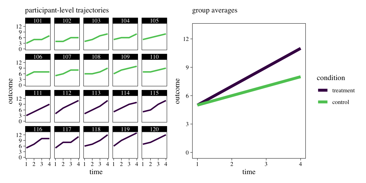
The series of miniature plots on the left shows the trajectory of each participant’s raw data, over time. The larger plot on the right shows the average value for each of the experimental conditions, over time. Although there is some variation across individuals within experimental conditions, clear trends emerge. The plot on the right shows the experimental conditions had the same average values at baseline (t1), both conditions tended to increase over time, but the treatment condition showed larger changes over time, relative to the control condition.
What do we care about?
There are a lot of questions a clinical researcher might want to ask from data of this kind. If we narrow our focus to causal inference1 with regards to the treatment conditions, I think there are three fundamental questions we’d want to ask. They all have to do with change over time:
- How much did the participants in the control group change, on average?
- How much did the participants in the treatment group change, on average?
- What was the difference in change in the treatment group versus the control group, on average?
Ideally, we’d like to express our answers to these questions, particularly the third, in terms of a meaningfully defined effect size. That will be the goal of the remainder of this post and the next.
Warm up with just two time points
Before we put on our big-kid pants and start fitting longitudinal growth models, I recommend we follow Feingold’s approach and first focus on how we’d answer these questions with two-time-point data. If we were to drop the variables t2 and t3, these data would have the form of a pre/post experiment, which Feingold called an independent-groups pretest–posttest design (IGPP2,
2009, p. 46). A major reason to warm up in this way is because much of the work on effect sizes, from Cohen (
1988) and others (e.g.,
Cumming, 2012), has been in the context of cross-sectional and pre/post designs, such as the IGPP. Not only have the analytic strategies centered on these simple cases, but the effect sizes designed for these simple cases are the ones most readers are used to interpreting. One of the big points in Feingold’s paper is we should prefer it when the effect sizes for our longitudinal growth models have clear links to the traditional effect sizes. I am inclined to agree.
Data summaries.
To get a sense of the pre/post changes in the two conditions, a fine place to start is with summary statistics. Here we compute the means and standard deviations in the outcome variable for each condition at pre and post. We also throw in the means and standard deviations for the change scores, t4-t1.
d %>%
  pivot_longer(cols = c(t1, t4, `t4-t1`),
               names_to = "variable") %>%
  group_by(variable, condition) %>%
  summarise(mean = mean(value),
            sd   = sd(value))
## # A tibble: 6 × 4
## # Groups:   variable [3]
##   variable condition  mean    sd
##   <chr>    <chr>     <dbl> <dbl>
## 1 t1       control       5 1.15
## 2 t1       treatment     5 1.15
## 3 t4       control       8 1.15
## 4 t4       treatment    11 1.15
## 5 t4-t1    control       3 0.816
## 6 t4-t1    treatment     6 0.816
Feingold displayed most of these statistics in his Table 1 (p. 46). Make special note of how consistent the \(SD\) values are. This will become important in the second post. Anyway, now we’re ready to start defining the effect sizes. We’ll start with the unstandardized kind.
Unstandardized mean differences.
The version of Cohen’s \(d\) we’re ultimately working up to is a special kind of standardized effect size. Yet not all effect sizes are standardized. In cases where the metric of the dependent variable is inherently meaningful, Pek and Flora (
2018) actually recommend researchers use unstandardized effect sizes. Say we thought the data in this example had values that were inherently meaningful. We could answer the three research questions, above, directly with sample statistics. Here we answer the first two questions by focusing on the means of the change scores, by experimental condition.
d %>%
  group_by(condition) %>%
  summarise(mean_change = mean(`t4-t1`))
## # A tibble: 2 × 2
##   condition mean_change
##   <chr>           <dbl>
## 1 control             3
## 2 treatment           6
To answer to our final question, we simply compute the difference between those two change scores.
6 - 3
## [1] 3
Although the average values in both groups changed over time, the participants in the treatment condition changed 3 units more, on average, than those in the control condition. Is that difference meaningful? At the moment, it seems hard to say because these data are not actually on an inherently meaningful metric. The whole thing is made up and abstract. We might be better off by using a standardized effect size, instead.
Standardized mean differences.
The approach above works great if the outcome variable is inherently meaningful and if we have no interest in comparing these results with studies on different outcome variables. In reality, clinical researchers often use sum scores from self-report questionnaires as their primary outcome variables and these scores take on seemingly arbitrary values. Say you work in depression research. There are numerous questionnaires designed to measure depression (e.g., Fried, 2017) and their sum scores are all scaled differently. The problem is even worse if you’d like to compare two different kinds of outcomes, such as depression and anxiety. This is where standardized effect sizes come in.
Since we are focusing on the data from the first and last time points, we can use conventional summary-statistic oriented strategies to compute the standardized mean differences. In the literature, you’ll often find standardized mean differences referred to as a Cohen’s \(d\), named after the late
Jacob Cohen. I suspect what isn’t always appreciated is that there are many ways to compute \(d\) and that “Cohen’s \(d\)” can both refer to the general family of standardized mean differences or to a specific kind of standardized mean difference. In addition to Cohen’s original (
1988) work, I think Geoff Cumming walked this out nicely in Chapter 11 of his (
2012) text. Here we’ll consider two versions of \(d\) from Feingold’s paper:
Two effect sizes can be calculated from an IGPP design, one using the standard deviation of the change scores in the denominator and the other using the standard deviation of the raw scores ( Morris, 2008; Morris & DeShon, 2002):
where
\(SD_\text{change-T}\)is the [standard deviation for the change scores]3 for the treatment group and\(SD_\text{change-T}\)is the [standard deviation for the change scores] for the control group. (If homogeneity of variance across conditions is assumed, each of these terms can be replaced by\(SD_\text{change}\)).where
\(M_\text{change-T}\)is the mean of the change scores for the treatment group,\(M_\text{change-C}\)is the mean of change scores for the control group,\(SD_\text{raw(pre-T)}\)is the pretest\(SD\)for the treatment group, and\(SD_\text{raw(pre-C)}\)is the pretest\(SD\)for the control group. (If homogeneity of variance is assumed, each of the last two terms can be replaced by\(SD_\text{raw}\).) (p. 47)
We should practice computing these values by hand. First, we compute the group-level summary statistics and save each value separately for further use.
# group-level change score means
m_change_t <- filter(d, tx ==  "0.5") %>% summarise(m = mean(`t4-t1`)) %>% pull()  # 6
m_change_c <- filter(d, tx == "-0.5") %>% summarise(m = mean(`t4-t1`)) %>% pull()  # 3

# group-level change score sds
sd_change_t <- filter(d, tx ==  "0.5") %>% summarise(s = sd(`t4-t1`)) %>% pull()  # 0.8164966
sd_change_c <- filter(d, tx == "-0.5") %>% summarise(s = sd(`t4-t1`)) %>% pull()  # 0.8164966

# group-level baseline sds
sd_raw_pre_t <- filter(d, tx ==  "0.5") %>% summarise(s = sd(t1)) %>% pull()  # 1.154701
sd_raw_pre_c <- filter(d, tx == "-0.5") %>% summarise(s = sd(t1)) %>% pull()  # 1.154701
With all those values saved, here’s how we might use the first equation, above, to compute Feingold’s \(d_\text{IGPP-change}\).
(m_change_t / sd_change_t) - (m_change_c / sd_change_c)
## [1] 3.674235
In a similar way, here’s how we might the second equation to compute \(d_\text{IGPP-raw}\).
(m_change_t / sd_raw_pre_t) - (m_change_c / sd_raw_pre_c)
## [1] 2.598076
In most areas of psychology, \(d\)’s of this size would seem large. Whether researchers prefer the \(d_\text{IGPP-change}\) approach or the \(d_\text{IGPP-raw}\) approach, both return effect sizes in the form of a standardized difference of differences. The primary question is what values to standardize the differences by (i.e., which \(SD\) estimates might we place in the denominators). As discussed by both Feingold (
2009) and Cumming (
2012), researchers are at liberty to make rational decisions on how to standardize their variables, and thus how to compute \(d\). Whatever you decide for your research, just make sure you clarify your choice and your formulas for your audience.
Extensions.
This is about as far as we’re going to go with the IGPP version of Feingold’s synthetic data. But if you do end up with data of this kind or similar, there are other things to consider. Real brief, here are two:
It’s good to express uncertainty.
Just like any other statistical estimate, we should express the uncertainty in our effect sizes, somehow. In the seventh edition of the APA Publication Manual, we read: “whenever possible, provide a confidence interval for each effect size reported to indicate the precision of estimation of the effect size” [American Psychological Association (
2020), p. 89]4. Since the ultimate purpose of this mini blog series is to show how to compute effect sizes for multilevel growth models, I am not going to dive into this issue, here. We’re just warming up for the main event in the next post. But if you ever need to compute 95% CIs for \(d_\text{IGPP-change}\) or \(d_\text{IGPP-raw}\) based on IGPP data, check out Chapter 11 in Cumming (
2012)5.
There are many more \(d\)’s.
We’ve already mentioned there are several kinds of Cohen’s \(d\) effect sizes. With Feingold’s data, we practiced two: \(d_\text{IGPP-change}\) and \(d_\text{IGPP-raw}\). Feingold built his paper on the foundation of Morris & DeShon (
2002), which covered a larger variety of \(d\)’s suited for cross-sectional and pre/post designs with one or two experimental conditions. Morris and DeShon’s writing style was accessible and I liked their statistical notation. You might check out their paper and expand your \(d\) repertoire.
What we learned and what’s soon to come
In this first post, we learned:
- Effect sizes for experimental trials analyzed with multilevel growth models aren’t straightforward.
- Much of the effect size literature is based on simple cross-sectional or two-time-point designs with one or two groups.
- Effect sizes can be standardized or unstandardized.
- “Cohen’s
\(d\)” can refer to either a general class of standardized mean differences, or to a specific standardized mean differences. - As discussed in Feingold (
2009), the two effect sizes recommended for IGPP designs are
\(d_\text{IGPP-change}\)or\(d_\text{IGPP-raw}\), both of which can be computed with simple summary statistics.
Stay tuned for the second post in this series, where we’ll extend these skills to two-group experimental data with more than two time points. The multilevel growth model will make its grand appearance and it’ll just be great!
Session info
sessionInfo()
## R version 4.2.0 (2022-04-22)
## Platform: x86_64-apple-darwin17.0 (64-bit)
## Running under: macOS Big Sur/Monterey 10.16
##
## Matrix products: default
## BLAS:   /Library/Frameworks/R.framework/Versions/4.2/Resources/lib/libRblas.0.dylib
## LAPACK: /Library/Frameworks/R.framework/Versions/4.2/Resources/lib/libRlapack.dylib
##
## locale:
## [1] en_US.UTF-8/en_US.UTF-8/en_US.UTF-8/C/en_US.UTF-8/en_US.UTF-8
##
## attached base packages:
## [1] stats     graphics  grDevices utils     datasets  methods   base
##
## other attached packages:
##  [1] patchwork_1.1.2 forcats_0.5.1   stringr_1.4.1   dplyr_1.0.10
##  [5] purrr_0.3.4     readr_2.1.2     tidyr_1.2.1     tibble_3.1.8
##  [9] ggplot2_3.4.0   tidyverse_1.3.2
##
## loaded via a namespace (and not attached):
##  [1] lubridate_1.8.0     assertthat_0.2.1    digest_0.6.30
##  [4] utf8_1.2.2          R6_2.5.1            cellranger_1.1.0
##  [7] backports_1.4.1     reprex_2.0.2        evaluate_0.18
## [10] highr_0.9           httr_1.4.4          blogdown_1.15
## [13] pillar_1.8.1        rlang_1.0.6         googlesheets4_1.0.1
## [16] readxl_1.4.1        rstudioapi_0.13     jquerylib_0.1.4
## [19] rmarkdown_2.16      labeling_0.4.2      googledrive_2.0.0
## [22] munsell_0.5.0       broom_1.0.1         compiler_4.2.0
## [25] modelr_0.1.8        xfun_0.35           pkgconfig_2.0.3
## [28] htmltools_0.5.3     tidyselect_1.1.2    bookdown_0.28
## [31] viridisLite_0.4.1   fansi_1.0.3         crayon_1.5.2
## [34] tzdb_0.3.0          dbplyr_2.2.1        withr_2.5.0
## [37] grid_4.2.0          jsonlite_1.8.3      gtable_0.3.1
## [40] lifecycle_1.0.3     DBI_1.1.3           magrittr_2.0.3
## [43] scales_1.2.1        cli_3.4.1           stringi_1.7.8
## [46] cachem_1.0.6        farver_2.1.1        fs_1.5.2
## [49] xml2_1.3.3          bslib_0.4.0         ellipsis_0.3.2
## [52] generics_0.1.3      vctrs_0.5.0         tools_4.2.0
## [55] glue_1.6.2          hms_1.1.1           fastmap_1.1.0
## [58] yaml_2.3.5          colorspace_2.0-3    gargle_1.2.0
## [61] rvest_1.0.2         knitr_1.40          haven_2.5.1
## [64] sass_0.4.2
References
American Psychological Association. (2020). Publication manual of the American Psychological Association (Seventh Edition). American Psychological Association. https://apastyle.apa.org/products/publication-manual-7th-edition
Cohen, J. (1988). Statistical power analysis for the behavioral sciences. L. Erlbaum Associates. https://www.worldcat.org/title/statistical-power-analysis-for-the-behavioral-sciences/oclc/17877467
Cumming, G. (2012). Understanding the new statistics: Effect sizes, confidence intervals, and meta-analysis. Routledge. https://www.routledge.com/Understanding-The-New-Statistics-Effect-Sizes-Confidence-Intervals-and/Cumming/p/book/9780415879682
Feingold, A. (2009). Effect sizes for growth-modeling analysis for controlled clinical trials in the same metric as for classical analysis. Psychological Methods, 14(1), 43. https://doi.org/10.1037/a0014699
Fried, E. I. (2017). The 52 symptoms of major depression: Lack of content overlap among seven common depression scales. Journal of Affective Disorders, 208, 191–197. https://doi.org/10.1016/j.jad.2016.10.019
Gelman, A., Hill, J., & Vehtari, A. (2020). Regression and other stories. Cambridge University Press. https://doi.org/10.1017/9781139161879
Grolemund, G., & Wickham, H. (2017). R for data science. O’Reilly. https://r4ds.had.co.nz
Hoffman, L. (2015). Longitudinal analysis: Modeling within-person fluctuation and change (1 edition). Routledge. https://www.routledge.com/Longitudinal-Analysis-Modeling-Within-Person-Fluctuation-and-Change/Hoffman/p/book/9780415876025
Kelley, K., & Preacher, K. J. (2012). On effect size. Psychological Methods, 17(2), 137. https://doi.org/10.1037/a0028086
Kruschke, J. K. (2015). Doing Bayesian data analysis: A tutorial with R, JAGS, and Stan. Academic Press. https://sites.google.com/site/doingbayesiandataanalysis/
McElreath, R. (2020). Statistical rethinking: A Bayesian course with examples in R and Stan (Second Edition). CRC Press. https://xcelab.net/rm/statistical-rethinking/
McElreath, R. (2015). Statistical rethinking: A Bayesian course with examples in R and Stan. CRC press. https://xcelab.net/rm/statistical-rethinking/
Morris, S. B. (2008). Estimating effect sizes from pretest-posttest-control group designs. Organizational Research Methods, 11(2), 364–386. https://doi.org/10.1177/1094428106291059
Morris, S. B., & DeShon, R. P. (2002). Combining effect size estimates in meta-analysis with repeated measures and independent-groups designs. Psychological Methods, 7(1), 105. https://doi.org/10.1037/1082-989X.7.1.105
Pek, J., & Flora, D. B. (2018). Reporting effect sizes in original psychological research: A discussion and tutorial. Psychological Methods, 23(2), 208. https://doi.org/ https://doi.apa.org/fulltext/2017-10871-001.html
R Core Team. (2022). R: A language and environment for statistical computing. R Foundation for Statistical Computing. https://www.R-project.org/
Raudenbush, S. W., & Bryk, A. S. (2002). Hierarchical linear models: Applications and data analysis methods (Second Edition). SAGE Publications, Inc. https://us.sagepub.com/en-us/nam/hierarchical-linear-models/book9230
Singer, J. D., & Willett, J. B. (2003). Applied longitudinal data analysis: Modeling change and event occurrence. Oxford University Press, USA. https://oxford.universitypressscholarship.com/view/10.1093/acprof:oso/9780195152968.001.0001/acprof-9780195152968
Wickham, H. (2022). tidyverse: Easily install and load the ’tidyverse’. https://CRAN.R-project.org/package=tidyverse
Wickham, H., Averick, M., Bryan, J., Chang, W., McGowan, L. D., François, R., Grolemund, G., Hayes, A., Henry, L., Hester, J., Kuhn, M., Pedersen, T. L., Miller, E., Bache, S. M., Müller, K., Ooms, J., Robinson, D., Seidel, D. P., Spinu, V., … Yutani, H. (2019). Welcome to the tidyverse. Journal of Open Source Software, 4(43), 1686. https://doi.org/10.21105/joss.01686
-
If you are unfamiliar with causal inference and confused over why causal inference might lead us to limit our focus in this way, check out Chapters 18 through 21 in Gelman et al. ( 2020). ↩︎
-
I’m not in love with introducing this new acronym. But if we want to follow along with Feingold, we may as well get used to his term. ↩︎
-
In the original paper, Feingold used the term “mean change score” here as well as a bit later in the sentence. After reading this through several times and working through his examples, I’m confident these were typos. With technical material of this kind, it’s hard to avoid a typo or two. ↩︎
-
We Bayesians, of course, can forgive the frequentist bias in the wording of the APA’s otherwise sound recommendation. ↩︎
-
Could you compute Bayesian credible intervals for IGPP effect sizes by adjusting some of the strategies from my earlier blog post, Regression models for 2-timepoint non-experimental data? Yes, you could. ↩︎
- Posted on:
- January 26, 2021
- Length:
- 18 minute read, 3630 words