Effect sizes for experimental trials analyzed with multilevel growth models: Two of two

Version 1.1.0

Edited on December 12, 2022, to use the new as_draws_df() workflow.

Orientation

This post is the second and final installment of a two-part series. In the first post, we explored how one might compute an effect size for two-group experimental data with only \(2\) time points. In this second post, we fulfill our goal to show how to generalize this framework to experimental data collected over \(3+\) time points. The data and overall framework come from Feingold ( 2009).

I still make assumptions.

As with the first post, I make a handful of assumptions about your background knowledge. Though I won’t spell them out again, here, I should stress that you’ll want to be familiar with multilevel models to get the most out of this post. To brush up, I recommend Raudenbush & Bryk ( 2002), Singer & Willett ( 2003), or Hoffman ( 2015).

As before, all code is in R ( R Core Team, 2022). Here we load our primary R packages– brms ( Bürkner, 2017, 2018, 2022), tidybayes ( Kay, 2022), and the tidyverse ( Wickham et al., 2019; Wickham, 2022)–and adjust the global plotting theme defaults.

library(brms)
library(tidybayes)
library(tidyverse)

# adjust the global plotting theme
theme_set(
  theme_linedraw() +
    theme(text = element_text(family = "Times"),
          panel.grid = element_blank(),
          strip.text = element_text(margin = margin(b = 3, t = 3)))
)

We need data.

Once again, we use the tribble approach to enter the synthetic data Feingold displayed in his Table 1 (p. 46).

d <-
  tribble(
    ~id, ~tx, ~t1, ~t2, ~t3, ~t4,
    101, -0.5, 3, 5, 5,  7,
    102, -0.5, 4, 4, 6,  6,
    103, -0.5, 4, 5, 7,  8,
    104, -0.5, 5, 6, 6,  8,
    105, -0.5, 5, 6, 7,  8,
    106, -0.5, 5, 7, 7,  7,
    107, -0.5, 5, 6, 8,  8,
    108, -0.5, 6, 6, 7,  9,
    109, -0.5, 6, 8, 9,  10,
    110, -0.5, 7, 7, 8,  9,
    111,  0.5, 3, 5, 7,  9,
    112,  0.5, 4, 7, 9,  11,
    113,  0.5, 4, 6, 8,  11,
    114,  0.5, 5, 7, 9,  10,
    115,  0.5, 5, 6, 9,  11,
    116,  0.5, 5, 7, 10, 10,
    117,  0.5, 5, 8, 8,  11,
    118,  0.5, 6, 7, 9,  12,
    119,  0.5, 6, 9, 11, 13,
    120,  0.5, 7, 8, 10, 12
  ) %>% 
  mutate(`t4-t1`   = t4 - t1,
         condition = ifelse(tx == -0.5, "control", "treatment"))

# inspect the first six rows
head(d)

## # A tibble: 6 × 8
##      id    tx    t1    t2    t3    t4 `t4-t1` condition
##   <dbl> <dbl> <dbl> <dbl> <dbl> <dbl>   <dbl> <chr>    
## 1   101  -0.5     3     5     5     7       4 control  
## 2   102  -0.5     4     4     6     6       2 control  
## 3   103  -0.5     4     5     7     8       4 control  
## 4   104  -0.5     5     6     6     8       3 control  
## 5   105  -0.5     5     6     7     8       3 control  
## 6   106  -0.5     5     7     7     7       2 control

To reacquaint ourselves with the data, we might make a plot. Last time we plotted a subset of the individual trajectories next to the averages, by treatment group. Here we’ll superimpose all the individual-level trajectories atop the group averages.

d %>% 
  pivot_longer(t1:t4) %>% 
  mutate(time      = str_extract(name, "\\d") %>% as.double(),
         condition = ifelse(tx < 0, "tx = -0.5 (control)", "tx = 0.5 (treatment)")) %>% 
  
  ggplot(aes(x = time, y = value)) +
  stat_smooth(aes(color = condition),
              method = "lm", formula = 'y ~ x',
              se = F, linewidth = 4) +
  geom_line(aes(group = id),
            linewidth = 1/4) +
  scale_color_viridis_d(end = .75, direction = -1, breaks = NULL) +
  facet_wrap(~ condition)

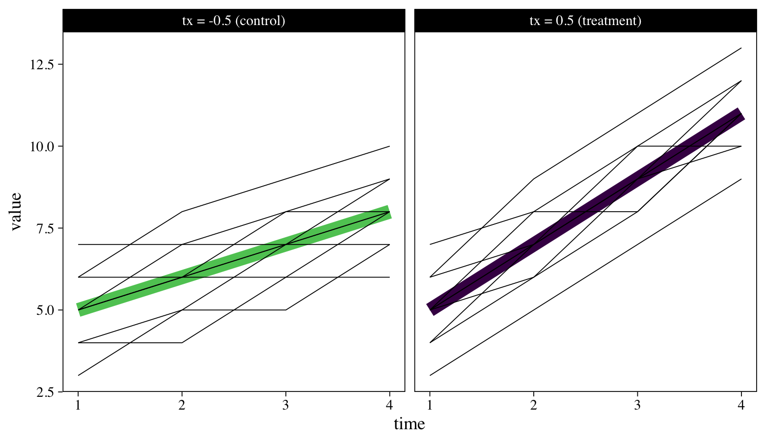
The thick lines are the group averages and the thinner lines are for the individual participants. Though participants tend to increase in both groups, those in the treatment condition appear to have increased at a more rapid pace. We want a standardized effect size that can capture those differences in a familiar metric. We’ll begin to explain what that will be, next.

Model

We need a framework.

Traditional analytic strategies, such as ordinary least squares (OLS) regression and the analysis of variance (ANOVA) framework, can work okay with data collected on one or two time points. In his ( 2009, 2013) work, which is the inspiration for this blog series, Feingold recommended what he called growth-modeling analysis (GMA) for data collected on \(3+\) time points. If you’re not familiar with the term GMA, it’s a longitudinal version of what others have called hierarchical linear models, mixed-effects models, random-effects models, or multilevel models. For longitudinal data, I’m fond of the term multilevel growth model, but you can use whatever term you like. If you’re interested, Raudenbush and Bryk touched on the historic origins of several of these terms in the first chapter of their ( 2002) text.

Though multilevel growth models, GMAs, have become commonplace in many applied areas, it’s not immediately obvious how to compute standardized effect sizes when one uses them. In his Discussion section, Feingold ( 2009, p. 49) pointed out this topic is missing from many text books and software user’s guides. For example, though I took five statistics courses in graduate school, one of which even focused on the longitudinal growth model, none of my courses covered how to compute an effect size in a longitudinal growth model and none of my text books covered the topic, either. It’s hard to expect researchers to use strategies we don’t bother to teach, which is the reason for this blog series.

We might walk out the framework with statistical notation. If we say our outcome variable \(y\) varies across \(i\) partitcipants and \(t\) time points, we might use Feingold’s Raudenbusch-&-Bryk-type notation to express our upcoming statistical model as

$$ \begin{align*} y_{ti} & = \beta_{00} + \beta_{01} (\text{treatment})_i + \beta_{10} (\text{time})_{ti} + \color{darkred}{\beta_{11}} (\text{treatment})_i (\text{time})_{ti} \\ & \;\;\; + [r_{0i} + r_{1i} (\text{time})_{ti} + e_{ti}], \end{align*} $$

where variance in \(y_{ti}\) is decomposed into the last three terms, \(r_{0i}\), \(r_{1i}\), and \(e_{ti}\). Here we follow the usual assumption that within-participant variance is normally distributed, \(e_{ti} \sim \operatorname N(0, \sigma_\epsilon^2)\), and the \(r_{\text{x}i}\) values follow a bivariate normal distribution,

$$ \begin{bmatrix} r_{0i} \ r_{1i} \end{bmatrix} \sim \operatorname N \left ( \begin{bmatrix} 0 \ 0 \end{bmatrix}, \begin{bmatrix} \tau_{00} & \tau_{01} \ \tau_{01} & \tau_{11} \end{bmatrix} \right ), $$

where the \(\tau\) terms on the diagonal are the variances and the off-diagonal \(\tau_{01}\) is their covariance. We’ll be fitting this model with Bayesian software, which means all parameters will be given prior distributions. But since our goal is to emphasize the effect size and the multilevel framework, I’m just going to use the brms default settings for the priors and will avoid expressing them in formal statistical notation¹.

In this model, the four \(\beta\) parameters are often called the “fixed effects,” or the population parameters. Our focal parameter will be \(\color{darkred}{\beta_{11}}\), which is why we marked it off in red. This parameter is the interaction between time and treatment condition. Put another way, \(\color{darkred}{\beta_{11}}\) is the difference in the average rate of change, by treatment. Once we fit our multilevel growth model, we will explore how one might transform the \(\color{darkred}{\beta_{11}}\) parameter into our desired effect size.

Fit the model.

As you’ll learn in any good multilevel text book, multilevel models typically require the data to be in the long format. Here we’ll transform our data into that format and call the results d_long.

# wrangle
d_long <-
  d %>% 
  pivot_longer(t1:t4, values_to = "y") %>% 
  mutate(time = str_extract(name, "\\d") %>% as.double()) %>% 
  mutate(time_f = (time * 2) - 5,
         time_c = time - mean(time),
         time0  = time - 1,
         time01 = (time - 1) / 3)

# what have we done?
head(d_long)

## # A tibble: 6 × 11
##      id    tx `t4-t1` condition name      y  time time_f time_c time0 time01
##   <dbl> <dbl>   <dbl> <chr>     <chr> <dbl> <dbl>  <dbl>  <dbl> <dbl>  <dbl>
## 1   101  -0.5       4 control   t1        3     1     -3   -1.5     0  0    
## 2   101  -0.5       4 control   t2        5     2     -1   -0.5     1  0.333
## 3   101  -0.5       4 control   t3        5     3      1    0.5     2  0.667
## 4   101  -0.5       4 control   t4        7     4      3    1.5     3  1    
## 5   102  -0.5       2 control   t1        4     1     -3   -1.5     0  0    
## 6   102  -0.5       2 control   t2        4     2     -1   -0.5     1  0.333

In the ( 2009) paper, Feingold mentioned he coded time as a factor which

was mean centered by using linear weights (-3, -1, 1, and 3 for T1 through T4, respectively) for a four-level design obtained from a table of orthogonal polynomials (Snedecor & Cochran, 1967) for the within-subjects (Level 1 in HLM terminology) facet of the analysis. (p. 47)

You can find this version of the time variable in the time_f column. However, I have no interest in modeling with time coded according to a scheme of orthogonal polynomials. But I do think it makes sense to center time or scale it so the lowest value is zero. You can find those versions of time in the time_c and time0 columns. The model, below, uses time0. Although this will change the scale of our model parameters relative to those in Feingold’s paper, it will have little influence on how we compute the effect size of interest.

Here’s how we might fit the multilevel growth model for the two treatment conditions with brms.

fit1 <-
  brm(data = d_long,
      family = gaussian,
      y ~ 1 + time0 + tx + time0:tx + (1 + time0 | id),
      cores = 4,
      seed = 1,
      control = list(adapt_delta = .85))

Review the parameter summary.

print(fit1)

##  Family: gaussian 
##   Links: mu = identity; sigma = identity 
## Formula: y ~ 1 + time0 + tx + time0:tx + (1 + time0 | id) 
##    Data: d_long (Number of observations: 80) 
##   Draws: 4 chains, each with iter = 2000; warmup = 1000; thin = 1;
##          total post-warmup draws = 4000
## 
## Group-Level Effects: 
## ~id (Number of levels: 20) 
##                      Estimate Est.Error l-95% CI u-95% CI Rhat Bulk_ESS Tail_ESS
## sd(Intercept)            1.08      0.23     0.74     1.63 1.00     1466     2084
## sd(time0)                0.09      0.07     0.00     0.25 1.00     1250     2274
## cor(Intercept,time0)    -0.07      0.51    -0.92     0.91 1.00     3696     2094
## 
## Population-Level Effects: 
##           Estimate Est.Error l-95% CI u-95% CI Rhat Bulk_ESS Tail_ESS
## Intercept     4.99      0.27     4.47     5.53 1.00     1099     1771
## time0         1.50      0.06     1.38     1.62 1.00     4311     2373
## tx           -0.01      0.56    -1.15     1.09 1.00     1117     1532
## time0:tx      1.00      0.12     0.76     1.24 1.00     4832     3164
## 
## Family Specific Parameters: 
##       Estimate Est.Error l-95% CI u-95% CI Rhat Bulk_ESS Tail_ESS
## sigma     0.57      0.06     0.47     0.69 1.00     3269     3137
## 
## Draws were sampled using sampling(NUTS). For each parameter, Bulk_ESS
## and Tail_ESS are effective sample size measures, and Rhat is the potential
## scale reduction factor on split chains (at convergence, Rhat = 1).

Everything looks fine. If you check them, the trace plots of the chains look good, too². If you execute the code below, you’ll see our primary results cohere nicely with the maximum likelihood results from the frequentist lme4 package.

lme4::lmer(data = d_long,
           y ~ 1 + time0 + tx + time0:tx + (1 + time0 | id)) %>% 
  summary()

Regardless on whether you focus on the output from brms or lme4, our coefficients will differ a bit from those Feingold reported because of our different scaling of the time variable. But from a high-level perspective, it’s the same model.

Unstandardized effect size.

Our interest lies in the time0:tx interaction, which is the unstandardized effect size for the “difference between the means of the slopes of the treatment and the control group” (p. 47). You might also describe this as a difference in differences. Here’s a focused summary of that coefficient, which Feingold called \(\beta_{11}\).

fixef(fit1)["time0:tx", ]

##  Estimate Est.Error      Q2.5     Q97.5 
## 0.9994403 0.1241458 0.7550637 1.2438976

Since there are three units of time between baseline (time0 == 0) and the final assessment point (time0 == 3), we can get the difference in pre/post differences by multiplying that \(\beta_{11}\) coefficient by 3.

fixef(fit1)["time0:tx", -2] * 3

## Estimate     Q2.5    Q97.5 
## 2.998321 2.265191 3.731693

Thinking back to the original wide-formatted d data, this value is the multilevel growth model version of the difference in change scores (t4-t1) in the treatment conditions, \(M_\text{change-T} - M_\text{change-C}\). Here compute that value by hand.

# group-level change score means
m_change_t <- filter(d, tx ==  "0.5") %>% summarise(m = mean(`t4-t1`)) %>% pull()  # 6
m_change_c <- filter(d, tx == "-0.5") %>% summarise(m = mean(`t4-t1`)) %>% pull()  # 3

# difference in change score means
m_change_t - m_change_c

## [1] 3

One of the reasons we went through the trouble of fitting a multilevel model is so we could accompany that difference in change scores with high-quality 95% intervals. Here they are in a coefficient plot.

data.frame(fixef(fit1)[, -2] * 3) %>% 
  rownames_to_column("coefficient") %>% 
  filter(coefficient == "time0:tx") %>% 
  
  ggplot(aes(x = Estimate, xmin = Q2.5, xmax = Q97.5, y = 0)) +
  geom_vline(xintercept = 0, linetype = 2) +
  geom_pointrange(fatten = 1) +
  scale_y_continuous(NULL, breaks = NULL) +
  xlab(expression("unstandardized difference in change scores"~(beta[1][1])))

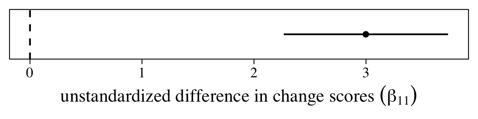
The population average could be anywhere from 2.25 to 3.75, but the best guess is it’s about 3. However, since the metric on this outcome variable is arbitrary (these data were simulated, remember), it’s hard to interpret how “large” this is. A standardized effect size can help.

We need to define the standardized mean difference for the multilevel growth model.

Based on Raudenbush & Liu ( 2001), Feingold presented two effect-size formulas for our multilevel growth model. The first, which he called \(d_\text{GMA-change}\), is on a completely different scale from any of the effect sizes mentioned in the first post (e.g., \(d_\text{IGPP-change}\) and \(d_\text{IGPP-raw}\)). Importantly, it turns out Raudenbush and Liu recommended their \(d_\text{GMA-change}\) formula should be used for power calculations, but not necessarily to convey the magnitude of an effect. Thus we will not consider it further³. Feingold reported the formula for their other effect size was

$$ d_\text{GMA-raw} = \beta_{11}(\text{time}) / SD_\text{raw}. $$

The \(\beta_{11}\) in Feingold’s equation is the multilevel interaction term between time and experimental condition–what we just visualized in a coefficient plot. The \((\text{time})\) part in the equation is a stand-in for the quantity of time units from the beginning of the study to the end point. Since our multilevel model used the time0 variable, which was 0 at baseline and 3 at the final time point, we would enter a 3 into the equation (i.e., \(3 - 0 = 3\)). The part of Feingold’s equation that’s left somewhat vague is what he meant by the denominator, \(SD_\text{raw}\). On page 47, he used the value of 1.15 in his example. Without any reference to experimental condition in the subscript, one might assume that value is the standard deviation for the criterion across all time points or, perhaps, just at baseline. It turns out that’s not the case.

# standard deviation for the criterion across all time points
d_long %>% 
  summarise(sd = sd(y))

## # A tibble: 1 × 1
##      sd
##   <dbl>
## 1  2.22

# standard deviation for the criterion at baseline
d_long %>% 
  filter(time == 1) %>% 
  summarise(sd = sd(y))

## # A tibble: 1 × 1
##      sd
##   <dbl>
## 1  1.12

For this particular data set, the value Feingold used is the same as the standard deviation for either of the experimental conditions at baseline.

sd_raw_pre_t <- filter(d, tx ==  "0.5") %>% summarise(s = sd(t1)) %>% pull()  # treatment baseline SD
sd_raw_pre_c <- filter(d, tx == "-0.5") %>% summarise(s = sd(t1)) %>% pull()  # control baseline SD

sd_raw_pre_c

## [1] 1.154701

sd_raw_pre_t

## [1] 1.154701

But since he didn’t use a subscript, I suspect Feingold meant to convey a pooled standard deviation, following the equation

$$SD_\text{pooled} = \sqrt{\frac{SD_\text{raw(pre-T)}^2 + SD_\text{raw(pre-C)}^2}{2}},$$

which is a sample version of Cohen’s original equation 2.3.2 ( 1988, p. 44). Here’s how to compute the pooled standard deviation by hand, which we’ll save as sd_raw_pre_p.

sd_raw_pre_p <- sqrt((sd_raw_pre_c^2 + sd_raw_pre_t^2) / 2)
sd_raw_pre_p

## [1] 1.154701

Since Feingold’s synthetic data are a special case where \(SD_\text{raw(pre-T)} = SD_\text{raw(pre-C)} = SD_\text{pooled}\), these distinctions might all seem dull and pedantic. Yet if your real-world data look anything like mine, this won’t be the case and you’ll need to understand how distinguish between and choose from among these options.

Another thing to consider is that whereas Feingold’s synthetic data have the desirable quality where the sample sizes are the same across the experimental conditions ($n_\text{T} = n_\text{C} = 10$), this won’t always be the case. If you end up with unbalanced experimental data, you might consider the sample-size weighted pooled standard deviation, \(SD_\text{pooled}^*\), which I believe has its origins in Hedges’ work ( 1981, p. 110). It follows the formula

$$SD_\text{pooled}^* = \sqrt{\frac{(n_\text{T} - 1)SD_\text{raw(pre-T)}^2 + (n_\text{C} - 1)SD_\text{raw(pre-C)}^2}{n_\text{T} + n_\text{C} - 2}}.$$

Here it is for Feingold’s data.

# define the sample sizes
n_t <- 10
n_c <- 10

# compute the sample size robust pooled SD
sqrt(((n_t - 1) * sd_raw_pre_c^2 + (n_c - 1) * sd_raw_pre_t^2) / (n_t + n_c - 2))

## [1] 1.154701

Again, in the special case of these synthetic data, \(SD_\text{pooled}^*\) happens to be the same value as \(SD_\text{pooled}\), which is also the same value as \(SD_\text{raw(pre-T)}\) and \(SD_\text{raw(pre-C)}\). This will not always the case with your real-world data. Choose your \(SD\) with care and make sure to report which ever formula you use. Don’t be coy with your effect-size calculations.

You may be wondering, though, whether you can use the standard deviations for one of the treatment conditions rather than a variant of the pooled standard deviation. Yes, you can. I think Cumming ( 2012, Chapter 11) did a nice job walking through this issue. For example, if we thought of our control condition as a true benchmark for what we’d expect at baseline, we could just use \(SD_\text{raw(pre-C)}\) as our standardizer. This is sometimes referred to as a Glass’ \(d\) or Glass’ \(\Delta\). Whatever you choose and whatever you call it, just make sure to clearly define your standardizing formula for your audience.

Therefore, if we use \(SD_\text{raw(pre-C)}\) (sd_raw_pre_c) as our working value, we can compute \(d_\text{GMA-raw}\) as follows.

fixef(fit1)["time0:tx", 1] * 3 / sd_raw_pre_c

## [1] 2.596622

Within the Bayesian framework, we can get a full posterior distribution for the standardized version of \(\beta_{11}\), \(d_\text{GMA-raw}\), by working directly with all the posterior draws.

as_draws_df(fit1) %>% 
  mutate(d = `b_time0:tx` * 3 / sd_raw_pre_p) %>% 
  
  ggplot(aes(x = d, y = 0)) +
  geom_vline(xintercept = 0, linetype = 2) +
  stat_halfeye(.width = .95) +
  scale_y_continuous(NULL, breaks = NULL) +
  xlab(expression(italic(d)[GMA-raw]~("standardized difference in change scores")))

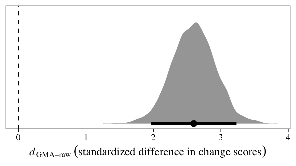
The population average could be anywhere from 2 to 3.25, but the best guess is it’s about 2.5. In my field (clinical psychology), this would be considered a very large effect size. Anyway, here are the numeric values for the posterior median and percentile-based 95% interval.

as_draws_df(fit1) %>% 
  mutate(d = `b_time0:tx` * 3 / sd_raw_pre_p) %>% 
  median_qi(d) %>% 
  mutate_if(is.double, round, digits = 2)

## # A tibble: 1 × 6
##       d .lower .upper .width .point .interval
##   <dbl>  <dbl>  <dbl>  <dbl> <chr>  <chr>    
## 1   2.6   1.96   3.23   0.95 median qi

Another way to compute this is to work with the model formula and the posterior samples from the fixed effects.

as_draws_df(fit1) %>% 
  # simplify the output
  select(starts_with("b_")) %>% 
  # compute the treatment-level means for pre and post
  mutate(m_pre_t  = b_Intercept + b_time0 * 0 + b_tx *  0.5 + `b_time0:tx`* 0 *  0.5,
         m_pre_c  = b_Intercept + b_time0 * 0 + b_tx * -0.5 + `b_time0:tx`* 0 * -0.5,
         m_post_t = b_Intercept + b_time0 * 3 + b_tx *  0.5 + `b_time0:tx`* 3 *  0.5,
         m_post_c = b_Intercept + b_time0 * 3 + b_tx * -0.5 + `b_time0:tx`* 3 * -0.5) %>% 
  # compute the treatment-level change scores
  mutate(m_change_t = m_post_t - m_pre_t,
         m_change_c = m_post_c - m_pre_c) %>% 
  # compute the difference of differences
  mutate(beta_11 = m_change_t - m_change_c) %>% 
  # compute the multilevel effect size
  mutate(d_GAM_raw = beta_11 / sd_raw_pre_c) %>% 
  # wrangle and summarize
  pivot_longer(m_pre_t:d_GAM_raw) %>% 
  group_by(name) %>% 
  mean_qi(value) %>% 
  mutate_if(is.double, round, digits = 2)

## # A tibble: 8 × 7
##   name       value .lower .upper .width .point .interval
##   <chr>      <dbl>  <dbl>  <dbl>  <dbl> <chr>  <chr>    
## 1 beta_11     3      2.27   3.73   0.95 mean   qi       
## 2 d_GAM_raw   2.6    1.96   3.23   0.95 mean   qi       
## 3 m_change_c  3      2.5    3.5    0.95 mean   qi       
## 4 m_change_t  6      5.48   6.53   0.95 mean   qi       
## 5 m_post_c    8      7.22   8.78   0.95 mean   qi       
## 6 m_post_t   11.0   10.3   11.7    0.95 mean   qi       
## 7 m_pre_c     5      4.2    5.78   0.95 mean   qi       
## 8 m_pre_t     4.99   4.26   5.73   0.95 mean   qi

Notice how the summary values in the rows for beta_11 and d_GAM_raw match up with those we computed, above.

You may want options.

Turns out there’s an other way to compute the standardized mean difference for experimental longitudinal data. You can just fit the model to the standardized data. As with our approach, above, the trick is to make sure you standardized the data with a defensible standardizer. I recommend you default to the pooled standard deviation at baseline ($SD_\text{pooled}$). To do so, we first compute the weighted mean at baseline.

# group-level baseline means
m_raw_pre_t <- filter(d, tx ==  "0.5") %>% summarise(m = mean(`t1`)) %>% pull()
m_raw_pre_c <- filter(d, tx ==  "-0.5") %>% summarise(m = mean(`t1`)) %>% pull()

# weighted (pooled) baseline mean
m_raw_pre_p <- (m_raw_pre_t * n_t + m_raw_pre_c * n_c) / (n_t + n_c)

m_raw_pre_p

## [1] 5

Next use the weighted baseline mean and the pooled baseline standard deviation to standardize the data, saving the results as z.

d_long <-
  d_long %>% 
  mutate(z = (y - m_raw_pre_p) / sd_raw_pre_p)

Now just fit a multilevel growth model with our new standardized variable z as the criterion.

fit2 <-
  brm(data = d_long,
      family = gaussian,
      z ~ 1 + time0 + tx + time0:tx + (1 + time0 | id),
      cores = 4,
      seed = 1)

Check the parameter summary.

print(fit2)

##  Family: gaussian 
##   Links: mu = identity; sigma = identity 
## Formula: z ~ 1 + time0 + tx + time0:tx + (1 + time0 | id) 
##    Data: d_long (Number of observations: 80) 
##   Draws: 4 chains, each with iter = 2000; warmup = 1000; thin = 1;
##          total post-warmup draws = 4000
## 
## Group-Level Effects: 
## ~id (Number of levels: 20) 
##                      Estimate Est.Error l-95% CI u-95% CI Rhat Bulk_ESS Tail_ESS
## sd(Intercept)            0.94      0.20     0.64     1.40 1.00     1435     2257
## sd(time0)                0.08      0.06     0.00     0.23 1.01     1197     2220
## cor(Intercept,time0)    -0.07      0.50    -0.92     0.89 1.00     4118     2701
## 
## Population-Level Effects: 
##           Estimate Est.Error l-95% CI u-95% CI Rhat Bulk_ESS Tail_ESS
## Intercept    -0.00      0.24    -0.47     0.46 1.00     1194     1948
## time0         1.30      0.06     1.19     1.41 1.00     5196     2624
## tx            0.01      0.48    -0.94     0.96 1.01     1136     1695
## time0:tx      0.87      0.11     0.65     1.09 1.00     4680     3001
## 
## Family Specific Parameters: 
##       Estimate Est.Error l-95% CI u-95% CI Rhat Bulk_ESS Tail_ESS
## sigma     0.50      0.05     0.41     0.60 1.00     3452     2858
## 
## Draws were sampled using sampling(NUTS). For each parameter, Bulk_ESS
## and Tail_ESS are effective sample size measures, and Rhat is the potential
## scale reduction factor on split chains (at convergence, Rhat = 1).

As before, our focal parameter is \(\beta_{11}\).

fixef(fit2)["time0:tx", -2]

##  Estimate      Q2.5     Q97.5 
## 0.8668416 0.6487548 1.0881314

But since our data are coded such that baseline is time0 == 0 and the final time point is time0 == 3, we’ll need to multiply that coefficient by 3 to get the effect size in the pre/post metric.

fixef(fit2)["time0:tx", -2] * 3

## Estimate     Q2.5    Q97.5 
## 2.600525 1.946264 3.264394

There is it, within simulation variance of the effect size from the last section. Let’s compare them with a coefficient plot.

rbind(fixef(fit1)["time0:tx", -2] * 3 / sd_raw_pre_p,
      fixef(fit2)["time0:tx", -2] * 3) %>% 
  data.frame() %>% 
  mutate(data = c("unstandardized data", "standardized data")) %>% 
  
  ggplot(aes(x = Estimate, xmin = Q2.5, xmax = Q97.5, y = data)) +
  geom_vline(xintercept = 0, linetype = 2) +
  geom_pointrange(fatten = 1) +
  labs(x = expression(italic(d)[GMA-raw]~("standardized difference in change scores")),
       y = NULL) +
  theme(axis.text.y = element_text(hjust = 0))

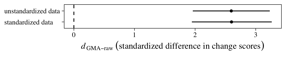
Yep, they’re pretty much the same.

Sum up

Yes, one can compute a standardized mean difference effect size for experimental data analyzed with a multilevel growth model. The focal parameter is the treatment-time interaction, what we called \(\beta_{11}\). The trick is to divide that parameter by the pooled standard deviation at baseline. This will put the effect size, what Feingold called \(d_\text{GMA-raw}\), into a conventional Cohen’s-$d$-type metric. But be mindful that this method may require you to multiply the effect by a number that corrects for how you have scaled the time variable. In the example we worked through, we multiplied by 3.

As an alternative workflow, you can also fit the model on data that were standardized using the pooled standard deviation at baseline. This will automatically put the \(\beta_{11}\) in the effect-size metric. But as with the other method, you still might have to correct for how you scaled the time variable.

Though we’re not covering it, here, Feingold ( 2013) extended this framework to other contexts. For example, he discussed how to apply it to data with nonlinear trends and to models with other covariates. Just know the foundation is right here:

$$ d_\text{GMA-raw} = \beta_{11}(\text{time}) / SD_\text{raw}. $$

Session info

sessionInfo()

## R version 4.2.0 (2022-04-22)
## Platform: x86_64-apple-darwin17.0 (64-bit)
## Running under: macOS Big Sur/Monterey 10.16
## 
## Matrix products: default
## BLAS:   /Library/Frameworks/R.framework/Versions/4.2/Resources/lib/libRblas.0.dylib
## LAPACK: /Library/Frameworks/R.framework/Versions/4.2/Resources/lib/libRlapack.dylib
## 
## locale:
## [1] en_US.UTF-8/en_US.UTF-8/en_US.UTF-8/C/en_US.UTF-8/en_US.UTF-8
## 
## attached base packages:
## [1] stats     graphics  grDevices utils     datasets  methods   base     
## 
## other attached packages:
##  [1] forcats_0.5.1   stringr_1.4.1   dplyr_1.0.10    purrr_0.3.4     readr_2.1.2     tidyr_1.2.1     tibble_3.1.8   
##  [8] ggplot2_3.4.0   tidyverse_1.3.2 tidybayes_3.0.2 brms_2.18.0     Rcpp_1.0.9     
## 
## loaded via a namespace (and not attached):
##   [1] readxl_1.4.1         backports_1.4.1      plyr_1.8.7           igraph_1.3.4         splines_4.2.0       
##   [6] svUnit_1.0.6         crosstalk_1.2.0      TH.data_1.1-1        rstantools_2.2.0     inline_0.3.19       
##  [11] digest_0.6.30        htmltools_0.5.3      fansi_1.0.3          magrittr_2.0.3       checkmate_2.1.0     
##  [16] googlesheets4_1.0.1  tzdb_0.3.0           modelr_0.1.8         RcppParallel_5.1.5   matrixStats_0.62.0  
##  [21] xts_0.12.1           sandwich_3.0-2       prettyunits_1.1.1    colorspace_2.0-3     rvest_1.0.2         
##  [26] ggdist_3.2.0         haven_2.5.1          xfun_0.35            callr_3.7.3          crayon_1.5.2        
##  [31] jsonlite_1.8.3       lme4_1.1-31          survival_3.4-0       zoo_1.8-10           glue_1.6.2          
##  [36] gtable_0.3.1         gargle_1.2.0         emmeans_1.8.0        distributional_0.3.1 pkgbuild_1.3.1      
##  [41] rstan_2.21.7         abind_1.4-5          scales_1.2.1         mvtnorm_1.1-3        DBI_1.1.3           
##  [46] miniUI_0.1.1.1       viridisLite_0.4.1    xtable_1.8-4         stats4_4.2.0         StanHeaders_2.21.0-7
##  [51] DT_0.24              httr_1.4.4           htmlwidgets_1.5.4    threejs_0.3.3        arrayhelpers_1.1-0  
##  [56] posterior_1.3.1      ellipsis_0.3.2       pkgconfig_2.0.3      loo_2.5.1            farver_2.1.1        
##  [61] sass_0.4.2           dbplyr_2.2.1         utf8_1.2.2           labeling_0.4.2       tidyselect_1.1.2    
##  [66] rlang_1.0.6          reshape2_1.4.4       later_1.3.0          munsell_0.5.0        cellranger_1.1.0    
##  [71] tools_4.2.0          cachem_1.0.6         cli_3.4.1            generics_0.1.3       broom_1.0.1         
##  [76] ggridges_0.5.3       evaluate_0.18        fastmap_1.1.0        yaml_2.3.5           processx_3.8.0      
##  [81] knitr_1.40           fs_1.5.2             nlme_3.1-159         mime_0.12            projpred_2.2.1      
##  [86] xml2_1.3.3           compiler_4.2.0       bayesplot_1.9.0      shinythemes_1.2.0    rstudioapi_0.13     
##  [91] gamm4_0.2-6          reprex_2.0.2         bslib_0.4.0          stringi_1.7.8        highr_0.9           
##  [96] ps_1.7.2             blogdown_1.15        Brobdingnag_1.2-8    lattice_0.20-45      Matrix_1.4-1        
## [101] nloptr_2.0.3         markdown_1.1         shinyjs_2.1.0        tensorA_0.36.2       vctrs_0.5.0         
## [106] pillar_1.8.1         lifecycle_1.0.3      jquerylib_0.1.4      bridgesampling_1.1-2 estimability_1.4.1  
## [111] httpuv_1.6.5         R6_2.5.1             bookdown_0.28        promises_1.2.0.1     gridExtra_2.3       
## [116] codetools_0.2-18     boot_1.3-28          colourpicker_1.1.1   MASS_7.3-58.1        gtools_3.9.3        
## [121] assertthat_0.2.1     withr_2.5.0          shinystan_2.6.0      multcomp_1.4-20      hms_1.1.1           
## [126] mgcv_1.8-40          parallel_4.2.0       grid_4.2.0           coda_0.19-4          minqa_1.2.5         
## [131] rmarkdown_2.16       googledrive_2.0.0    shiny_1.7.2          lubridate_1.8.0      base64enc_0.1-3     
## [136] dygraphs_1.1.1.6

References

Bürkner, P.-C. (2017). brms: An R package for Bayesian multilevel models using Stan. Journal of Statistical Software, 80(1), 1–28. https://doi.org/10.18637/jss.v080.i01
Bürkner, P.-C. (2018). Advanced Bayesian multilevel modeling with the R package brms. The R Journal, 10(1), 395–411. https://doi.org/10.32614/RJ-2018-017
Bürkner, P.-C. (2021). brms reference manual, Version 2.15.0. https://CRAN.R-project.org/package=brms/brms.pdf
Bürkner, P.-C. (2022). brms: Bayesian regression models using ’Stan’. https://CRAN.R-project.org/package=brms
Cohen, J. (1988). Statistical power analysis for the behavioral sciences. L. Erlbaum Associates. https://www.worldcat.org/title/statistical-power-analysis-for-the-behavioral-sciences/oclc/17877467
Cumming, G. (2012). Understanding the new statistics: Effect sizes, confidence intervals, and meta-analysis. Routledge. https://www.routledge.com/Understanding-The-New-Statistics-Effect-Sizes-Confidence-Intervals-and/Cumming/p/book/9780415879682
Feingold, A. (2009). Effect sizes for growth-modeling analysis for controlled clinical trials in the same metric as for classical analysis. Psychological Methods, 14(1), 43. https://doi.org/10.1037/a0014699
Feingold, A. (2013). A regression framework for effect size assessments in longitudinal modeling of group differences. Review of General Psychology, 17(1), 111–121. https://doi.org/10.1037/a0030048
Hedges, L. V. (1981). Distribution theory for Glass’s estimator of effect size and related estimators. Journal of Educational Statistics, 6(2), 107–128. https://doi.org/10.3102/10769986006002107
Hoffman, L. (2015). Longitudinal analysis: Modeling within-Person fluctuation and change (1 edition). Routledge. https://www.routledge.com/Longitudinal-Analysis-Modeling-Within-Person-Fluctuation-and-Change/Hoffman/p/book/9780415876025
Kay, M. (2023). tidybayes: Tidy data and ’geoms’ for Bayesian models. https://CRAN.R-project.org/package=tidybayes
R Core Team. (2022). R: A language and environment for statistical computing. R Foundation for Statistical Computing. https://www.R-project.org/
Raudenbush, S. W., & Bryk, A. S. (2002). Hierarchical linear models: Applications and data analysis methods (Second Edition). SAGE Publications, Inc. https://us.sagepub.com/en-us/nam/hierarchical-linear-models/book9230
Raudenbush, S. W., & Liu, X.-F. (2001). Effects of study duration, frequency of observation, and sample size on power in studies of group differences in polynomial change. Psychological Methods, 6(4), 387. https://doi.org/10.1037/1082-989X.6.4.387
Singer, J. D., & Willett, J. B. (2003). Applied longitudinal data analysis: Modeling change and event occurrence. Oxford University Press, USA. https://oxford.universitypressscholarship.com/view/10.1093/acprof:oso/9780195152968.001.0001/acprof-9780195152968
Wickham, H. (2022). tidyverse: Easily install and load the ’tidyverse’. https://CRAN.R-project.org/package=tidyverse
Wickham, H., Averick, M., Bryan, J., Chang, W., McGowan, L. D., François, R., Grolemund, G., Hayes, A., Henry, L., Hester, J., Kuhn, M., Pedersen, T. L., Miller, E., Bache, S. M., Müller, K., Ooms, J., Robinson, D., Seidel, D. P., Spinu, V., … Yutani, H. (2019). Welcome to the tidyverse. Journal of Open Source Software, 4(43), 1686. https://doi.org/10.21105/joss.01686
-
If you’re curious about our priors, fit the models on your computer and then execute
fit1$prior. To learn more about brms default priors, spend some time with the brms reference manual ( Bürkner, 2021). ↩︎ -
If you’re not into the whole Bayesian framework I’m using, you can just ignore the part about trace plots and chains. If you’re into it, execute
plot(fit1). ↩︎ -
Really. If you are interested in communicating your research results to others, do not mess with the
\(d_\text{GMA-change}\). It’s on a totally different metric from the conventional Cohen’s\(d\)and you’ll just end up confusing people. ↩︎
- Posted on:
- April 22, 2021
- Length:
- 24 minute read, 4919 words