Multilevel models and the index-variable approach
By A. Solomon Kurz
December 9, 2020
Version 1.1.0
Edited on December 16, 2022, to use the new as_draws_df() workflow.
The set-up
PhD candidate Huaiyu Liu recently reached out with a question about how to analyze clustered data. Liu’s basic setup was an experiment with four conditions. The dependent variable was binary, where success = 1, fail = 0. Each participant completed multiple trials under each of the four conditions. The catch was Liu wanted to model those four conditions with a multilevel model using the index-variable approach McElreath advocated for in the second edition of his text ( McElreath, 2020a).
Like any good question, this one got my gears turning. Thanks, Liu! The purpose of this post will be to show how to model data like this two different ways.
I make assumptions.
In this post, I’m presuming you are familiar with Bayesian multilevel models and with logistic regression. All code is in R ( R Core Team, 2022), with healthy doses of the tidyverse ( Wickham et al., 2019; Wickham, 2022). The statistical models will be fit with brms ( Bürkner, 2017, 2018, 2022). We’ll also make a little use of the tidybayes ( Kay, 2022) and rethinking ( McElreath, 2020b) packages. If you need to shore up, I list some educational resources at the end of the post.
Load the primary packages.
library(tidyverse)
library(brms)
library(tidybayes)
Data
The data for Liu’s question had the same basic structure as the chimpanzees data from the rethinking package. Happily, it’s also the case that Liu wanted to fit a model that was very similar to model m14.3 from Chapter 14 of McElreath’s text. Here we’ll load the data and wrangle a little.
data(chimpanzees, package = "rethinking")
d <- chimpanzees
rm(chimpanzees)

# wrangle
d <-
  d %>%
  mutate(actor = factor(actor),
         treatment = factor(1 + prosoc_left + 2 * condition),
         # this will come in handy, later
         labels    = factor(treatment,
                            levels = 1:4,
                            labels = c("r/n", "l/n", "r/p", "l/p")))

glimpse(d)
## Rows: 504
## Columns: 10
## $ actor        <fct> 1, 1, 1, 1, 1, 1, 1, 1, 1, 1, 1, 1, 1, 1, 1, 1, 1, 1, 1, 1, 1, 1, 1, 1, 1, 1,…
## $ recipient    <int> NA, NA, NA, NA, NA, NA, NA, NA, NA, NA, NA, NA, NA, NA, NA, NA, NA, NA, NA, N…
## $ condition    <int> 0, 0, 0, 0, 0, 0, 0, 0, 0, 0, 0, 0, 0, 0, 0, 0, 0, 0, 0, 0, 0, 0, 0, 0, 0, 0,…
## $ block        <int> 1, 1, 1, 1, 1, 1, 2, 2, 2, 2, 2, 2, 3, 3, 3, 3, 3, 3, 4, 4, 4, 4, 4, 4, 5, 5,…
## $ trial        <int> 2, 4, 6, 8, 10, 12, 14, 16, 18, 20, 22, 24, 26, 28, 30, 32, 34, 36, 38, 40, 4…
## $ prosoc_left  <int> 0, 0, 1, 0, 1, 1, 1, 1, 0, 0, 0, 1, 0, 1, 0, 1, 1, 0, 1, 0, 0, 0, 1, 1, 0, 0,…
## $ chose_prosoc <int> 1, 0, 0, 1, 1, 1, 0, 0, 1, 1, 0, 0, 0, 1, 1, 1, 0, 1, 1, 0, 0, 1, 1, 0, 1, 0,…
## $ pulled_left  <int> 0, 1, 0, 0, 1, 1, 0, 0, 0, 0, 1, 0, 1, 1, 0, 1, 0, 0, 1, 1, 1, 0, 1, 0, 0, 1,…
## $ treatment    <fct> 1, 1, 2, 1, 2, 2, 2, 2, 1, 1, 1, 2, 1, 2, 1, 2, 2, 1, 2, 1, 1, 1, 2, 2, 1, 1,…
## $ labels       <fct> r/n, r/n, l/n, r/n, l/n, l/n, l/n, l/n, r/n, r/n, r/n, l/n, r/n, l/n, r/n, l/…
The focal variable will be pulled_left, which is binary and coded yes = 1, no = 0. We have four experimental conditions, which are indexed 1 through 4 in the treatment variable. The shorthand labels for those conditions are saved as labels. These data are simple in that there are only seven participants, who are indexed in the actor column.
Within the generalized linear model framework, we typically model binary variables with binomial likelihood1. When you use the conventional link function, you can call this logistic regression. When you have a binary variable, the parameter of interest is the probability of a 1 in your criterion variable. When you want a quick sample statistic, you can estimate those probabilities with the mean. To get a sense of the data, here are the sample probabilities pulled_left == 1 for each of our seven participants, by the four levels of treatment.
d %>%
  mutate(treatment = str_c("treatment ", treatment)) %>%
  group_by(actor, treatment) %>%
  summarise(p = mean(pulled_left) %>% round(digits = 2)) %>%
  pivot_wider(values_from = p, names_from = treatment) %>%
  knitr::kable()
| actor | treatment 1 | treatment 2 | treatment 3 | treatment 4 |
|---|---|---|---|---|
| 1 | 0.33 | 0.50 | 0.28 | 0.56 |
| 2 | 1.00 | 1.00 | 1.00 | 1.00 |
| 3 | 0.28 | 0.61 | 0.17 | 0.33 |
| 4 | 0.33 | 0.50 | 0.11 | 0.44 |
| 5 | 0.33 | 0.56 | 0.28 | 0.50 |
| 6 | 0.78 | 0.61 | 0.56 | 0.61 |
| 7 | 0.78 | 0.83 | 0.94 | 1.00 |
Models
We are going to analyze these data two kinds of multilevel models. The first way is the direct analogue to McElreath’s model m14.3; it’ll be a multilevel model using the index-variable approach for the population-level intercepts. The second way is a multilevel Bayesian alternative to the ANOVA, based on Kruschke’s (
2015) text.
However, some readers might benefit from a review of what I even mean by the “index-variable” approach. This approach is uncommon in my field of clinical psychology, for example. So before we get down to business, we’ll clear that up by contrasting it with the widely-used dummy-variable approach.
Warm-up with the simple index-variable model.
Let’s forget the multilevel model for a moment. One of the more popular ways to use a categorical predictor variable is with the dummy-variable approach. Say we wanted to predict our criterion variable pulled_left with treatment, which is a four-category nominal variable. If we denote the number of categories \(K\), treatment is a \(K = 4\) nominal variable. The dummy-variable approach would be to break treatment into \(K - 1\) binary variables, which we’d simultaneously enter into the model. Say we broke treatment into three dummies with the following code.
d <-
  d %>%
  mutate(d2 = if_else(treatment == 2, 1, 0),
         d3 = if_else(treatment == 3, 1, 0),
         d4 = if_else(treatment == 4, 1, 0))
The dummy variables d2, d3, and d4 would capture the four levels of treatment like so:
d %>%
  distinct(treatment, d2, d3, d4)
##   treatment d2 d3 d4
## 1         1  0  0  0
## 2         2  1  0  0
## 3         3  0  1  0
## 4         4  0  0  1
Here d2 == 1 only when treatment == 2. Similarly, d3 == 1 only when treatment == 3 and d4 == 1 only when treatment == 4. When treatment == 1, all three dummies are 0, which makes treatment == 1 the reference category.
You can write out the statistical model using these \(K - 1\) dummies as
$$
\begin{align*} \text{left_pull}_i & \sim \operatorname{Binomial}(n_i = 1, p_i) \\ \operatorname{logit} (p_i) & = \beta_0 + \beta_1 \text{d2}_i + \beta_2 \text{d3}_i + \beta_3 \text{d4}_i, \end{align*}
$$
where \(\beta_0\) is both the “intercept” and the expected value for the first level of treatment. \(\beta_1\) is the expected change in value, relative to \(\beta_0\), for the second level of treatment. In the same way, \(\beta_2\) and \(\beta_3\) are changes relative to \(\beta_0\) for the third and fourth levels of treatment, respectively.
The index-variable approach takes a different stance. Rather than dividing treatment into dummies, one simply allows each level of treatment to have its own intercept. You can write that in statistical notation as
$$
\begin{align*} \text{left_pull}_i & \sim \operatorname{Binomial}(n_i = 1, p_i) \\ \operatorname{logit} (p_i) & = \gamma_{\text{treatment}[i]}, \end{align*}
$$
where the \(\text{treatment}[i]\) subscript indicates the different levels of treatment, which vary across cases \(i\), each get their own \(\gamma\) parameter. Because treatment has four levels, we end up with four \(\gamma\)’s: \(\gamma_1\), \(\gamma_2\), \(\gamma_3\), and \(\gamma_4\). When you model intercepts in this way, none of the levels of treatment end up as the reference category and none of the other levels of treatment are parameterized in terms of deviations from the reference category. Each intercept is estimated in its own terms.
Quick note on notation: There’s nothing special about using the letter \(\gamma\) for our index variable. We could just as easily have used \(\alpha\), \(\beta\), \(\xi\), or whatever. The only reason I’m using \(\gamma\), here, is because that’s what McElreath used for his model m14.3.
If you’d like more practice with dummy variables, McElreath lectured on them here. If you’d like to hear McElreath walk out index variables a bit more, you can find that lecture here.
McElreath’s approach.
Okay, now we’re up to speed on what Liu meant by wanting to fit a model with the index-variable approach, let’s see what that looks like in a multilevel model.
The statistical model.
Here’s how we might express McElreath’s index-variable approach to these data in statistical notation:
$$
\begin{align*} \text{left_pull}_i & \sim \operatorname{Binomial}(n_i = 1, p_i) \\ \operatorname{logit} (p_i) & = \gamma_{\text{treatment}[i]} + \alpha_{\text{actor}[i], \text{treatment}[i]} \\ \gamma_j & \sim \operatorname{Normal}(0, 1), \;\;\; \text{for } j = 1, \dots, 4 \\ \begin{bmatrix} \alpha_{j, 1} \\ \alpha_{j, 2} \\ \alpha_{j, 3} \\ \alpha_{j, 4} \end{bmatrix} & \sim \operatorname{MVNormal} \begin{pmatrix} \begin{bmatrix} 0 \\ 0 \\ 0 \\ 0 \end{bmatrix}, \mathbf \Sigma_\text{actor} \end{pmatrix} \\ \mathbf \Sigma_\text{actor} & = \mathbf{S_\alpha R_\alpha S_\alpha} \\ \sigma_{\alpha, [1]}, \dots, \sigma_{\alpha, [4]} & \sim \operatorname{Exponential}(1) \\ \mathbf R_\alpha & \sim \operatorname{LKJ}(2). \end{align*}
$$
In this model, we have four population-level intercepts, \(\gamma_1, \dots, \gamma_4\), one for each of the four levels of treatment. This is one of the critical features required by Liu’s question. actor is our higher-level grouping variable. The third line spells out the priors for those four \(\gamma\)’s. Though they all get the same prior in this model, you could use different priors for each, if you wanted.
Going back to the second line, the term \(\alpha_{\text{actor}[i], \text{treatment}[i]}\) is meant to convey that each of the treatment effects can vary by actor. We can–and should–do this because each of our participants experienced each of the four levels of treatment many times. The fourth line containing the \(\operatorname{MVNormal}(\cdot)\) operator might look intimidating. The vector on the left is just a way to list those four actor-level deviations we just mentioned. We’ll be treating them much the same way you might treat a random intercept and slope in a multilevel growth model. That is, we presume they follow a multivariate normal distribution. Since these are all deviations, the 4-dimensional mean vector in our multivariate normal distribution contains four zeros. The spread around those zeros are controlled by the variance/covariance matrix \(\Sigma_\text{actor}\). In the next line, we learn that \(\Sigma_\text{actor}\) can be decomposed into two terms, \(\mathbf S_\alpha\) and \(\mathbf R_\alpha\)2. It may not yet be clear by the notation, but \(\mathbf S_\alpha\) is a \(4 \times 4\) diagonal matrix of standard deviations,
$$ \mathbf S_\alpha = \begin{bmatrix} \sigma_{\alpha, [1]} & 0 & 0 & 0 \ 0 & \sigma_{\alpha, [2]} & 0 & 0 \ 0 & 0 & \sigma_{\alpha, [3]} & 0 \ 0 & 0 & 0 & \sigma_{\alpha, [4]} \end{bmatrix}. $$
In a similar way, \(\mathbf R_\alpha\) is a \(4 \times 4\) correlation matrix,
$$ \mathbf R_\alpha = \begin{bmatrix} 1 & \rho_{\alpha, [1, 2]} & \rho_{\alpha, [1, 3]} & \rho_{\alpha, [1, 4]} \ \rho_{\alpha, [2, 1]} & 1 & \rho_{\alpha, [2, 3]} & \rho_{\alpha, [2, 4]} \ \rho_{\alpha, [3, 1]} & \rho_{\alpha, [3, 2]} & 1 & \rho_{\alpha, [3, 4]} \ \rho_{\alpha, [4, 1]} & \rho_{\alpha, [4, 2]} & \rho_{\alpha, [4, 3]} & 1 \end{bmatrix}. $$
As we see in the sixth line, all the \(\sigma_\alpha\) parameters have individual \(\operatorname{Exponential}(1)\) priors. The final line shows the \(\mathbf R_\alpha\) matrix has the \(\operatorname{LKJ}(2)\) prior. Though you could certainly use different priors, here we’re sticking close to those McElreath used in his text.
Fit the model.
Though the statistical model might look intimidating, we can fit it pretty easily with brms::brm(). We’ll call this fit1.
fit1 <-
  brm(data = d,
      family = binomial,
      pulled_left | trials(1) ~ 0 + treatment + (0 + treatment | actor),
      prior = c(prior(normal(0, 1), class = b),
                prior(exponential(1), class = sd),
                prior(lkj(2), class = cor)),
      cores = 4, seed = 1)
From a syntax perspective, the important parts were the two occurrences of 0 + treatment in the model formula line. The first occurrence was how we told brms we wanted our population-level intercept to be indexed by the four levels of treatment. The second occurrence was where we told brms we wanted those to vary across our seven levels of actor.
Check the model summary.
print(fit1)
##  Family: binomial
##   Links: mu = logit
## Formula: pulled_left | trials(1) ~ 0 + treatment + (0 + treatment | actor)
##    Data: d (Number of observations: 504)
##   Draws: 4 chains, each with iter = 2000; warmup = 1000; thin = 1;
##          total post-warmup draws = 4000
##
## Group-Level Effects:
## ~actor (Number of levels: 7)
##                            Estimate Est.Error l-95% CI u-95% CI Rhat Bulk_ESS Tail_ESS
## sd(treatment1)                 1.36      0.49     0.67     2.56 1.00     2285     2681
## sd(treatment2)                 0.89      0.39     0.33     1.87 1.00     2542     3059
## sd(treatment3)                 1.84      0.56     1.00     3.21 1.00     3262     2563
## sd(treatment4)                 1.54      0.60     0.71     3.02 1.00     2766     2630
## cor(treatment1,treatment2)     0.43      0.28    -0.20     0.87 1.00     3040     2979
## cor(treatment1,treatment3)     0.53      0.25    -0.04     0.90 1.00     2885     2505
## cor(treatment2,treatment3)     0.48      0.27    -0.14     0.89 1.00     2921     2972
## cor(treatment1,treatment4)     0.44      0.27    -0.16     0.87 1.00     3144     3078
## cor(treatment2,treatment4)     0.43      0.28    -0.20     0.87 1.00     3134     3264
## cor(treatment3,treatment4)     0.57      0.25    -0.01     0.92 1.00     3231     2817
##
## Population-Level Effects:
##            Estimate Est.Error l-95% CI u-95% CI Rhat Bulk_ESS Tail_ESS
## treatment1     0.23      0.48    -0.71     1.22 1.00     1902     2258
## treatment2     0.66      0.36    -0.10     1.38 1.00     2488     2145
## treatment3    -0.03      0.57    -1.17     1.13 1.00     2767     2629
## treatment4     0.70      0.52    -0.37     1.74 1.00     2739     2255
##
## Draws were sampled using sampling(NUTS). For each parameter, Bulk_ESS
## and Tail_ESS are effective sample size measures, and Rhat is the potential
## scale reduction factor on split chains (at convergence, Rhat = 1).
If you look at the lower level of the output, the four levels in the ‘Population-Level Effects’ section are the four levels of \(\gamma_{\text{treatment}[i]}\) from our statistical formula. If you look above at the ‘Group-Level Effects’ section, the four lines beginning with “sd” correspond to our four \(\sigma_{\alpha, [1]}, \dots, \sigma_{\alpha, [4]}\) parameters. The correlations among those are depicted in the six rows beginning with “cor,” which correspond to the elements within the \(\mathbf R_\alpha\) matrix.
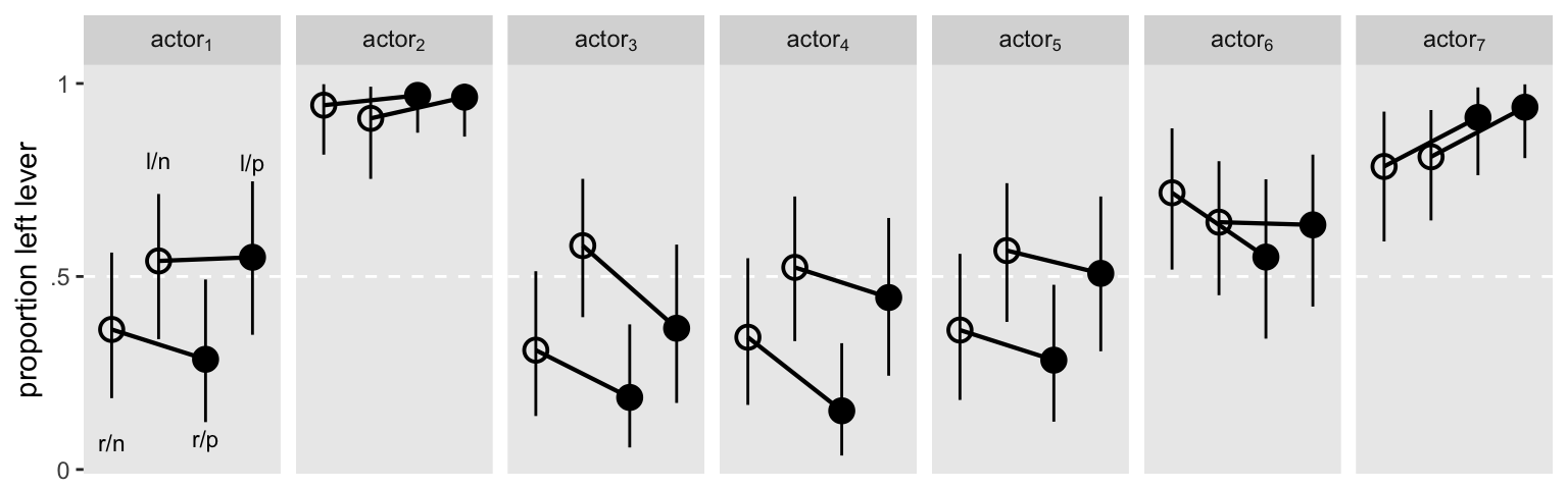
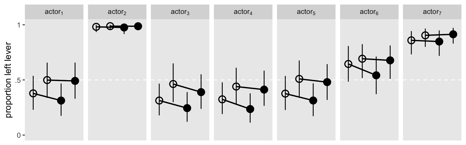
It might help if we visualized the model in a plot. Here are the results depicted in a streamlined version of McElreath’s Figure 14.7 ( McElreath, 2020a, p. 452).
# for annotation
text <-
  distinct(d, labels) %>%
  mutate(actor = "actor[1]",
         prop  = c(.07, .8, .08, .795))

# define the new data
nd <-
  d %>%
  distinct(actor, condition, labels, prosoc_left, treatment)

# get the fitted draws
fitted(fit1,
       newdata = nd) %>%
  data.frame() %>%
  bind_cols(nd) %>%
  mutate(actor     = str_c("actor[", actor, "]"),
         condition = factor(condition)) %>%

  # plot!
  ggplot(aes(x = labels)) +
  geom_hline(yintercept = .5, color = "white", linetype = 2) +
  # posterior predictions
  geom_line(aes(y = Estimate, group = prosoc_left),
            size = 3/4) +
  geom_pointrange(aes(y = Estimate, ymin = Q2.5, ymax = Q97.5, shape = condition),
                  fill = "transparent", fatten = 10, size = 1/3, show.legend = F) +
  # annotation for the conditions
  geom_text(data = text,
            aes(y = prop, label = labels),
            size = 3) +
  scale_shape_manual(values = c(21, 19)) +
  scale_x_discrete(NULL, breaks = NULL) +
  scale_y_continuous("proportion left lever", breaks = 0:2 / 2, labels = c("0", ".5", "1")) +
  theme(panel.grid = element_blank()) +
  facet_wrap(~actor, nrow = 1, labeller = label_parsed)
## Warning: Using `size` aesthetic for lines was deprecated in ggplot2 3.4.0.
## ℹ Please use `linewidth` instead.
Here’s an alternative version, this time faceting by treatment.
fitted(fit1,
       newdata = nd) %>%
  data.frame() %>%
  bind_cols(nd) %>%
  # add the gamma summaries
  left_join(
    tibble(treatment = as.character(1:4),
       gamma = inv_logit_scaled(fixef(fit1)[, 1])),
    by = "treatment"
  )  %>%
  mutate(treatment = str_c("treatment[", treatment, "]")) %>%

  # plot!
  ggplot(aes(x = reorder(actor, Estimate), y = Estimate, ymin = Q2.5, ymax = Q97.5)) +
  geom_hline(aes(yintercept = gamma),
             color = "white") +
  geom_pointrange(size = 1/3) +
  scale_x_discrete(breaks = NULL) +
  labs(x = "actor, rank orderred by their average probability",
       y = "probability of pulling the lever") +
  theme(panel.grid = element_blank()) +
  facet_wrap(~treatment, nrow = 1, labeller = label_parsed)
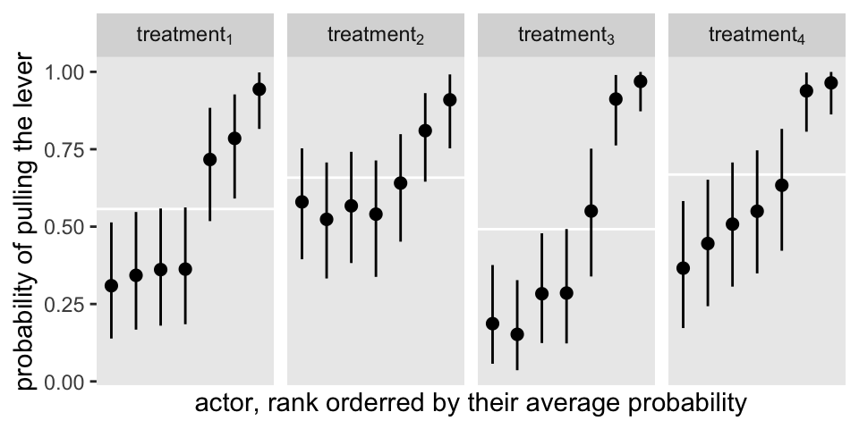
The horizontal white lines mark off the posterior means for the \(\gamma_{\text{treatment}[i]}\) parameters.
Kruschke’s approach.
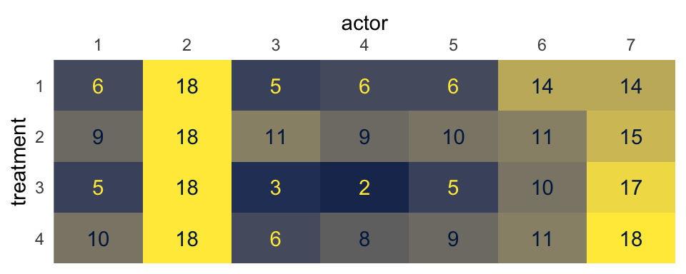
One way to think about our pulled_left data is they are grouped by two factors. The first factor is the experimental condition, treatment. The second factor is participant, actor. Now imagine you arrange the number of times pulled_left == 1 within the cells of a \(2 \times 2\) contingency table where the four levels of the treatment factor are in the rows and the seven levels of actor are in the columns. Here’s what that might look like in a tile plot.
d %>%
  group_by(actor, treatment) %>%
  summarise(count = sum(pulled_left)) %>%
  mutate(treatment = factor(treatment, levels = 4:1)) %>%

  ggplot(aes(x = actor, y = treatment, fill = count, label = count)) +
  geom_tile() +
  geom_text(aes(color = count > 6)) +
  scale_color_viridis_d(option = "E", direction = -1, breaks = NULL) +
  scale_fill_viridis_c(option = "E", limits = c(0, 18), breaks = NULL) +
  scale_x_discrete(position = "top", expand = c(0, 0)) +
  scale_y_discrete(expand = c(0, 0)) +
  theme(axis.ticks = element_blank())
With this arrangement, we can model \(\text{left_pull}_i \sim \operatorname{Binomial}(n_i = 1, p_i)\), with three hierarchical grouping factors. The first will be actor, the second will be treatment, and the third will be their interaction. Kruschke gave a general depiction of this kind of statistical model in Figure 20.23 of his text (
Kruschke, 2015, p. 588). However, I generally prefer expressing my models using statistical notation similar to McElreath. Though I’m not exactly sure how McElreath would express a model like this, here’s my best attempt using his style of notation:
$$
\begin{align*} \text{left_pull}_i & \sim \operatorname{Binomial}(n_i = 1, p_i) \\ \operatorname{logit} (p_i) & = \gamma + \alpha_{\text{actor}[i]} + \alpha_{\text{treatment}[i]} + \alpha_{\text{actor}[i] \times \text{treatment}[i]} \\ \gamma & \sim \operatorname{Normal}(0, 1) \\ \alpha_\text{actor} & \sim \operatorname{Normal}(0, \sigma_\text{actor}) \\ \alpha_\text{treatment} & \sim \operatorname{Normal}(0, \sigma_\text{treatment}) \\ \alpha_{\text{actor} \times \text{treatment}} & \sim \operatorname{Normal}(0, \sigma_{\text{actor} \times \text{treatment}}) \\ \sigma_\text{actor} & \sim \operatorname{Exponential}(1) \\ \sigma_\text{treatment} & \sim \operatorname{Exponential}(1) \\ \sigma_{\text{actor} \times \text{treatment}} & \sim \operatorname{Exponential}(1). \end{align*}
$$
Here \(\gamma\) is our overall intercept and the three \(\alpha_{\text{<group>}[i]}\) terms are our multilevel deviations around that overall intercept. Notice that because \(\gamma\) nas no \(j\) index, we are not technically using the index variable approach we discussed earlier in this post. But we are still indexing the four levels of treatment by way of higher-level deviations depicted by the \(\alpha_{\text{treatment}[i]}\) and \(\alpha_{\text{actor}[i] \times \text{treatment}[i]}\) parameters in the second line. In contrast to our first model based on McElreath’s work, notice our three \(\alpha_{\text{<group>}[i]}\) term are all modeled as univariate normal. This makes this model an extension of the cross-classified model.
Fit the second model.
Here’s how to fit the model with brms. We’ll call it fit2.
fit2 <-
  brm(data = d,
      family = binomial,
      pulled_left | trials(1) ~ 1 + (1 | actor) + (1 | treatment) + (1 | actor:treatment),
      prior = c(prior(normal(0, 1), class = Intercept),
                prior(exponential(1), class = sd)),
      cores = 4, seed = 1,
      control = list(adapt_delta = .85))
Check the summary.
print(fit2)
##  Family: binomial
##   Links: mu = logit
## Formula: pulled_left | trials(1) ~ 1 + (1 | actor) + (1 | treatment) + (1 | actor:treatment)
##    Data: d (Number of observations: 504)
##   Draws: 4 chains, each with iter = 2000; warmup = 1000; thin = 1;
##          total post-warmup draws = 4000
##
## Group-Level Effects:
## ~actor (Number of levels: 7)
##               Estimate Est.Error l-95% CI u-95% CI Rhat Bulk_ESS Tail_ESS
## sd(Intercept)     1.97      0.64     1.07     3.52 1.00     1435     2502
##
## ~actor:treatment (Number of levels: 28)
##               Estimate Est.Error l-95% CI u-95% CI Rhat Bulk_ESS Tail_ESS
## sd(Intercept)     0.24      0.18     0.01     0.66 1.00     1453     1867
##
## ~treatment (Number of levels: 4)
##               Estimate Est.Error l-95% CI u-95% CI Rhat Bulk_ESS Tail_ESS
## sd(Intercept)     0.55      0.36     0.08     1.46 1.00     1217     1056
##
## Population-Level Effects:
##           Estimate Est.Error l-95% CI u-95% CI Rhat Bulk_ESS Tail_ESS
## Intercept     0.47      0.61    -0.75     1.70 1.00     1204     1979
##
## Draws were sampled using sampling(NUTS). For each parameter, Bulk_ESS
## and Tail_ESS are effective sample size measures, and Rhat is the potential
## scale reduction factor on split chains (at convergence, Rhat = 1).
With a model like this, a natural first question is: Where is the variance at? We can answer that by comparing the three lines in the output from the ‘Group-Level Effects’ section. It might be easier if we plotted the posteriors for those \(\sigma_\text{<group>}\) parameters, instead.
library(tidybayes)

as_draws_df(fit2) %>%
  select(starts_with("sd")) %>%
  set_names(str_c("sigma[", c("actor", "actor~X~treatment", "treatment"), "]")) %>%
  pivot_longer(everything()) %>%
  mutate(name = factor(name,
                       levels = str_c("sigma[", c("actor~X~treatment", "treatment", "actor"), "]"))) %>%

  ggplot(aes(x = value, y = name)) +
  stat_halfeye(.width = .95, size = 1/2) +
  scale_y_discrete(NULL, labels = ggplot2:::parse_safe,
                   expand = expansion(add = 0.1)) +
  xlab("marginal posterior (log-odds scale)") +
  theme(axis.text.y = element_text(hjust = 0),
        axis.ticks.y = element_blank(),
        panel.grid = element_blank())
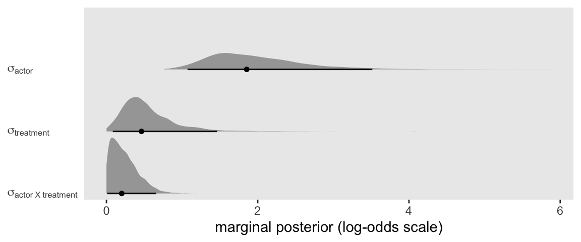
It looks like most of the action was between the seven actors. But there was some variation among the four levels of treatment and even the interaction between the two factors wasn’t completely pushed against zero.
Okay, here’s an alternative version of the first plot from fit1, above.
fitted(fit2,
       newdata = nd) %>%
  data.frame() %>%
  bind_cols(nd) %>%
  mutate(actor     = str_c("actor[", actor, "]"),
         condition = factor(condition)) %>%

  # plot!
  ggplot(aes(x = labels)) +
  geom_hline(yintercept = .5, color = "white", linetype = 2) +
  # posterior predictions
  geom_line(aes(y = Estimate, group = prosoc_left),
            size = 3/4) +
  geom_pointrange(aes(y = Estimate, ymin = Q2.5, ymax = Q97.5, shape = condition),
                  fill = "transparent", fatten = 10, size = 1/3, show.legend = F) +
  scale_shape_manual(values = c(21, 19)) +
  scale_x_discrete(NULL, breaks = NULL) +
  scale_y_continuous("proportion left lever", limits = 0:1,
                     breaks = 0:2 / 2, labels = c("0", ".5", "1")) +
  theme(panel.grid = element_blank()) +
  facet_wrap(~actor, nrow = 1, labeller = label_parsed)
The two models made similar predictions.
Why not make the horse race official?
Just for kicks and giggles, we’ll compare the two models with the LOO.
fit1 <- add_criterion(fit1, criterion = "loo")
fit2 <- add_criterion(fit2, criterion = "loo")

# LOO differences
loo_compare(fit1, fit2) %>% print(simplify = F)
##      elpd_diff se_diff elpd_loo se_elpd_loo p_loo  se_p_loo looic  se_looic
## fit2    0.0       0.0  -266.8      9.5        12.0    0.6    533.6   19.1
## fit1   -4.6       3.1  -271.4      9.7        19.3    1.1    542.8   19.4
# LOO weights
model_weights(fit1, fit2, weights = "loo")
##        fit1        fit2
## 0.009760051 0.990239949
It looks like there’s a little bit of an edge for the Kruschke’s multilevel ANOVA model.
But what’s the difference, anyway?
Rather than attempt to chose one model based on information criteria, we might back up and focus on the conceptual differences between the two models.
Our first model, based on McElreath’s index-variable approach, explicitly emphasized the four levels of treatment. Each one got its own \(\gamma_j\). By modeling those \(\gamma_j\)’s with the multivariate normal distribution, we also got an explicit accounting of the \(4 \times 4\) correlation structure for those parameters.
Our second model, based on Kruschke’s multilevel ANOVA approach, took a more general perspective. By modeling actor, treatment and their interaction as higher-level grouping factors, fit2 conceptualized both participants and experimental conditions as coming from populations of potential participants and conditions, respectively. No longer are those four treatment levels inherently special. They’re just the four we happen to have in this iteration of the experiment. Were we to run the experiment again, after all, we might want to alter them a little. The \(\sigma_\text{treatment}\) and \(\sigma_{\text{actor} \times \text{treatment}}\) parameters can help give us a sense of how much variation we’d expect among other similar experimental conditions.
Since I’m not a chimpanzee researcher, I’m in no position to say which perspective is better for these data. At a predictive level, the models perform similarly. But if I were a researcher wanting to analyze these data or others with a similar structure, I’d want to think clearly about what kinds of points I’d want to make to my target audience. Would I want to make focused points about the four levels of treatment, or would it make sense to generalize from those four levels to other similar conditions? Each model has its rhetorical strengths and weaknesses.
Next steps
If you’re new to the Bayesian multilevel model, I recommend the introductory text by either McElreath ( McElreath, 2020a) or Kruschke ( Kruschke, 2015). I have ebook versions of both wherein I translated their code into the tidyverse style and fit their models with brms ( Kurz, 2020a, 2020b). Both McElreath and Kruschke have blogs ( here and here). Also, though it doesn’t cover the multilevel model, you can get a lot of practice with Bayesian regression with the new book by Gelman, Hill, and Vehtari ( 2020). And for more hot Bayesian regression talk, you always have the Stan forums, which even have a brms section.
Session info
sessionInfo()
## R version 4.2.0 (2022-04-22)
## Platform: x86_64-apple-darwin17.0 (64-bit)
## Running under: macOS Big Sur/Monterey 10.16
##
## Matrix products: default
## BLAS:   /Library/Frameworks/R.framework/Versions/4.2/Resources/lib/libRblas.0.dylib
## LAPACK: /Library/Frameworks/R.framework/Versions/4.2/Resources/lib/libRlapack.dylib
##
## locale:
## [1] en_US.UTF-8/en_US.UTF-8/en_US.UTF-8/C/en_US.UTF-8/en_US.UTF-8
##
## attached base packages:
## [1] stats     graphics  grDevices utils     datasets  methods   base
##
## other attached packages:
##  [1] tidybayes_3.0.2 brms_2.18.0     Rcpp_1.0.9      forcats_0.5.1   stringr_1.4.1   dplyr_1.0.10
##  [7] purrr_0.3.4     readr_2.1.2     tidyr_1.2.1     tibble_3.1.8    ggplot2_3.4.0   tidyverse_1.3.2
##
## loaded via a namespace (and not attached):
##   [1] readxl_1.4.1         backports_1.4.1      plyr_1.8.7           igraph_1.3.4
##   [5] svUnit_1.0.6         splines_4.2.0        crosstalk_1.2.0      TH.data_1.1-1
##   [9] rstantools_2.2.0     inline_0.3.19        digest_0.6.30        htmltools_0.5.3
##  [13] fansi_1.0.3          magrittr_2.0.3       checkmate_2.1.0      googlesheets4_1.0.1
##  [17] tzdb_0.3.0           modelr_0.1.8         RcppParallel_5.1.5   matrixStats_0.62.0
##  [21] xts_0.12.1           sandwich_3.0-2       prettyunits_1.1.1    colorspace_2.0-3
##  [25] rvest_1.0.2          ggdist_3.2.0         haven_2.5.1          xfun_0.35
##  [29] callr_3.7.3          crayon_1.5.2         jsonlite_1.8.3       lme4_1.1-31
##  [33] survival_3.4-0       zoo_1.8-10           glue_1.6.2           gtable_0.3.1
##  [37] gargle_1.2.0         emmeans_1.8.0        distributional_0.3.1 pkgbuild_1.3.1
##  [41] rstan_2.21.7         abind_1.4-5          scales_1.2.1         mvtnorm_1.1-3
##  [45] DBI_1.1.3            miniUI_0.1.1.1       viridisLite_0.4.1    xtable_1.8-4
##  [49] stats4_4.2.0         StanHeaders_2.21.0-7 DT_0.24              htmlwidgets_1.5.4
##  [53] httr_1.4.4           threejs_0.3.3        arrayhelpers_1.1-0   posterior_1.3.1
##  [57] ellipsis_0.3.2       pkgconfig_2.0.3      loo_2.5.1            farver_2.1.1
##  [61] sass_0.4.2           dbplyr_2.2.1         utf8_1.2.2           labeling_0.4.2
##  [65] tidyselect_1.1.2     rlang_1.0.6          reshape2_1.4.4       later_1.3.0
##  [69] munsell_0.5.0        cellranger_1.1.0     tools_4.2.0          cachem_1.0.6
##  [73] cli_3.4.1            generics_0.1.3       broom_1.0.1          ggridges_0.5.3
##  [77] evaluate_0.18        fastmap_1.1.0        yaml_2.3.5           processx_3.8.0
##  [81] knitr_1.40           fs_1.5.2             nlme_3.1-159         mime_0.12
##  [85] projpred_2.2.1       xml2_1.3.3           compiler_4.2.0       bayesplot_1.9.0
##  [89] shinythemes_1.2.0    rstudioapi_0.13      gamm4_0.2-6          reprex_2.0.2
##  [93] bslib_0.4.0          stringi_1.7.8        highr_0.9            ps_1.7.2
##  [97] blogdown_1.15        Brobdingnag_1.2-8    lattice_0.20-45      Matrix_1.4-1
## [101] nloptr_2.0.3         markdown_1.1         shinyjs_2.1.0        tensorA_0.36.2
## [105] vctrs_0.5.0          pillar_1.8.1         lifecycle_1.0.3      jquerylib_0.1.4
## [109] bridgesampling_1.1-2 estimability_1.4.1   httpuv_1.6.5         R6_2.5.1
## [113] bookdown_0.28        promises_1.2.0.1     gridExtra_2.3        codetools_0.2-18
## [117] boot_1.3-28          colourpicker_1.1.1   MASS_7.3-58.1        gtools_3.9.3
## [121] assertthat_0.2.1     withr_2.5.0          shinystan_2.6.0      multcomp_1.4-20
## [125] mgcv_1.8-40          parallel_4.2.0       hms_1.1.1            grid_4.2.0
## [129] coda_0.19-4          minqa_1.2.5          rmarkdown_2.16       googledrive_2.0.0
## [133] shiny_1.7.2          lubridate_1.8.0      base64enc_0.1-3      dygraphs_1.1.1.6
References
Bürkner, P.-C. (2021). Parameterization of response distributions in brms. https://CRAN.R-project.org/package=brms/vignettes/brms_families.html
Bürkner, P.-C. (2017). brms: An R package for Bayesian multilevel models using Stan. Journal of Statistical Software, 80(1), 1–28. https://doi.org/10.18637/jss.v080.i01
Bürkner, P.-C. (2018). Advanced Bayesian multilevel modeling with the R package brms. The R Journal, 10(1), 395–411. https://doi.org/10.32614/RJ-2018-017
Bürkner, P.-C. (2022). brms: Bayesian regression models using ’Stan’. https://CRAN.R-project.org/package=brms
Gelman, A., Hill, J., & Vehtari, A. (2020). Regression and other stories. Cambridge University Press. https://doi.org/10.1017/9781139161879
Kay, M. (2022). tidybayes: Tidy data and ’geoms’ for Bayesian models. https://CRAN.R-project.org/package=tidybayes
Kruschke, J. K. (2015). Doing Bayesian data analysis: A tutorial with R, JAGS, and Stan. Academic Press. https://sites.google.com/site/doingbayesiandataanalysis/
Kurz, A. S. (2020a). Doing Bayesian data analysis in brms and the tidyverse (version 0.3.0). https://bookdown.org/content/3686/
Kurz, A. S. (2020b). Statistical rethinking with brms, Ggplot2, and the tidyverse: Second edition (version 0.1.1). https://bookdown.org/content/4857/
McElreath, R. (2020a). Statistical rethinking: A Bayesian course with examples in R and Stan (Second Edition). CRC Press. https://xcelab.net/rm/statistical-rethinking/
McElreath, R. (2020b). rethinking R package. https://xcelab.net/rm/software/
R Core Team. (2022). R: A language and environment for statistical computing. R Foundation for Statistical Computing. https://www.R-project.org/
Wickham, H. (2022). tidyverse: Easily install and load the ’tidyverse’. https://CRAN.R-project.org/package=tidyverse
Wickham, H., Averick, M., Bryan, J., Chang, W., McGowan, L. D., François, R., Grolemund, G., Hayes, A., Henry, L., Hester, J., Kuhn, M., Pedersen, T. L., Miller, E., Bache, S. M., Müller, K., Ooms, J., Robinson, D., Seidel, D. P., Spinu, V., … Yutani, H. (2019). Welcome to the tidyverse. Journal of Open Source Software, 4(43), 1686. https://doi.org/10.21105/joss.01686
-
Given the data are coded 0/1, one could also use the Bernoulli likelihood ( Bürkner, 2021, Binary and count data models). I’m just partial to the binomial. ↩︎
-
This is the typical parameterization for multilevel models fit with brms. Though he used different notation, Bürkner spelled this all out in his ( 2017) overview paper, brms: An R package for Bayesian multilevel models using Stan. ↩︎
-
The careful reader might notice that the models Kruschke focused on in Chapter 20 were all based on the Gaussian likelihood. So in the most technical sense, the model in Figure 20.2 is not a perfect match to our
fit2. I’m hoping my readers might look past those details to see the more general point. For more practice, Section 24.2 and Section 24.3 of my translation of Kruschke’s text ( Kurz, 2020a) show variants of this model type using the Poisson likelihood. In Section 24.4 you can even find a variant using the aggregated binomial likelihood. ↩︎
- Posted on:
- December 9, 2020
- Length:
- 23 minute read, 4898 words