Bayesian meta-analysis in brms-II

Version 1.1.0

Edited on December 12, 2022, to use the new as_draws_df() workflow.

Preamble

In Section 14.3 of my ( 2020) translation of the first edition of McElreath’s ( 2015) Statistical rethinking, I included a bonus section covering Bayesian meta-analysis. For my ( 2020) translation of the second edition of the text ( McElreath, 2020), I’d like to include another section on the topic, but from a different perspective. The first time around, we focused on standardized mean differences. This time, I’d like to tackle odds ratios and, while we’re at it, give a little bit of a plug for open science practices.

The purpose of this post is to present a rough draft of the section. I intend to tack this section onto the end of Chapter 15 (Missing Data and Other Opportunities), which covers measurement error. If you have any constrictive criticisms, please pass them along either in the GitHub issues for the ebook or on Twitter.

Here’s the rough draft:

Summary Bonus: Bayesian meta-analysis with odds ratios

# these packages and setting alterations will already have been 
# opened and made before this section
library(tidyverse)
library(brms)
library(ggdark)
library(viridis)
library(broom)
library(tidybayes)

theme_set(
  dark_theme_bw() +
    theme(legend.position = "none",
          panel.grid = element_blank())
  )

# to reset the default ggplot2 theme to its default parameters,
# execute `ggplot2::theme_set(theme_gray())` and `ggdark::invert_geom_defaults()`

If your mind isn’t fully blown by those measurement-error and missing-data models, let’s keep building. As it turns out, meta-analyses are often just special kinds of multilevel measurement-error models. Thus, you can use brms::brm() to fit Bayesian meta-analyses, too.

Before we proceed, I should acknowledge that this section is heavily influenced by Matti Vourre’s great blog post, Meta-analysis is a special case of Bayesian multilevel modeling. Since neither editions of McElreath’s text directly address meta-analyses, we’ll also have to borrow a bit from Gelman, Carlin, Stern, Dunson, Vehtari, and Rubin’s ( 2013) Bayesian data analysis, Third edition.

How do meta-analyses fit into the picture?

Let Gelman and colleagues introduce the topic:

Discussions of meta-analysis are sometimes imprecise about the estimands of interest in the analysis, especially when the primary focus is on testing the null hypothesis of no effect in any of the studies to be combined. Our focus is on estimating meaningful parameters, and for this objective there appear to be three possibilities, accepting the overarching assumption that the studies are comparable in some broad sense. The first possibility is that we view the studies as identical replications of each other, in the sense we regard the individuals in all the studies as independent samples from a common population, with the same outcome measures and so on. A second possibility is that the studies are so different that the results of any one study provide no information about the results of any of the others. A third, more general, possibility is that we regard the studies as exchangeable but not necessarily either identical or completely unrelated; in other words we allow differences from study to study, but such that the differences are not expected a priori to have predictable effects favoring one study over another…. this third possibility represents a continuum between the two extremes, and it is this exchangeable model (with unknown hyperparameters characterizing the population distribution) that forms the basis of our Bayesian analysis…

The first potential estimand of a meta-analysis, or a hierarchically structured problem in general, is the mean of the distribution of effect sizes, since this represents the overall ‘average’ effect across all studies that could be regarded as exchangeable with the observed studies. Other possible estimands are the effect size in any of the observed studies and the effect size in another, comparable (exchangeable) unobserved study. (pp. 125–126, emphasis in the original)

The basic version of a Bayesian meta-analysis follows the form

$$y_j \sim \operatorname{Normal}(\theta_j, \sigma_j),$$

where \(y_j\) = the point estimate for the effect size of a single study, \(j\), which is presumed to have been a draw from a Normal distribution centered on \(\theta_j\). The data in meta-analyses are typically statistical summaries from individual studies. The one clear lesson from this chapter is that those estimates themselves come with error and those errors should be fully expressed in the meta-analytic model. The standard error from study \(j\) is specified \(\sigma_j\), which is also a stand-in for the standard deviation of the Normal distribution from which the point estimate was drawn. Do note, we’re not estimating \(\sigma_j\), here. Those values we take directly from the original studies.

Building on the model, we further presume that study \(j\) is itself just one draw from a population of related studies, each of which have their own effect sizes. As such, we presume \(\theta_j\) itself has a distribution following the form

$$\theta_j \sim \operatorname{Normal}(\mu, \tau),$$

where \(\mu\) is the meta-analytic effect (i.e., the population mean) and \(\tau\) is the variation around that mean, what you might also think of as \(\sigma_\tau\).

We need some data.

Our data in this section come from the second large-scale replication project by the Many Labs team ( Klein et al., 2018). Of the 28 studies replicated in the study, we will focus on the replication of the trolley experiment from Hauser et al. ( 2007). Here’s how the study was described by Klein and colleagues:

According to the principle of double effect, an act that harms other people is more morally permissible if the act is a foreseen side effect rather than the means to the greater good. Hauser et al. ( 2007) compared participants’ reactions to two scenarios to test whether their judgments followed this principle. In the foreseen-side-effect scenario, a person on an out-of-control train changed the train’s trajectory so that the train killed one person instead of five. In the greater-good scenario, a person pushed a fat man in front of a train, killing him, to save five people. Whereas \(89\%\) of participants judged the action in the foreseen-side-effect scenario as permissible \((95 \% \; \text{CI} = [87\%, 91\%]),\) only \(11\%\) of participants in the greater-good scenario judged it as permissible \((95 \% \; \text{CI} = [9\%, 13\%])\). The difference between the percentages was significant$, \chi^2(1, N = 2,646) = 1,615.96,$ \(p < .001,\) \(w = .78,\) \(d = 2.50,\) \(95 \% \; \text{CI} = [2.22, 2.86]\). Thus, the results provided evidence for the principle of double effect. (p. 459, emphasis in the original)

You can find supporting materials for the replication project on the Open Science Framework at https://osf.io/8cd4r/. The relevant subset of the data for the replication of Hauser et al. come from the Trolley Dilemma 1 (Hauser et al., 2007) folder within the OSFdata.zip ( https://osf.io/ag2pd/). I’ve downloaded the file and saved it on GitHub.

Here we load the data and call it h.

h <- 
  readr::read_csv("https://raw.githubusercontent.com/ASKurz/Statistical_Rethinking_with_brms_ggplot2_and_the_tidyverse_2_ed/master/data/Hauser_1_study_by_order_all_CLEAN_CASE.csv")

h <- 
  h %>% 
  mutate(y   = ifelse(variable == "Yes", 1, 0),
         loc = factor(Location,
                      levels = distinct(h, Location) %>% pull(Location),
                      labels = 1:59))

glimpse(h)

## Rows: 6,842
## Columns: 29
## $ uID              <dbl> 65, 68, 102, 126, 145, 263, 267, 298, 309, 318, 350, 356, 376, 431, 438, …
## $ variable         <chr> "Yes", "Yes", "Yes", "Yes", "Yes", "No", "Yes", "Yes", "No", "Yes", "Yes"…
## $ factor           <chr> "SideEffect", "SideEffect", "SideEffect", "SideEffect", "SideEffect", "Si…
## $ .id              <chr> "ML2_Slate1_Brazil__Portuguese_execution_illegal_r.csv", "ML2_Slate1_Braz…
## $ source           <chr> "brasilia", "brasilia", "brasilia", "wilfredlaur", "wilfredlaur", "ubc", …
## $ haus1.1          <dbl> 1, 1, 1, 1, 1, 2, 1, 1, 2, 1, 1, 1, 1, 1, 1, 2, 1, 1, 2, 1, 1, 2, 1, 1, 1…
## $ haus1.1t_1       <dbl> 39.054, 36.792, 56.493, 21.908, 25.635, 50.633, 58.661, 50.137, 51.717, 2…
## $ haus2.1          <dbl> NA, NA, NA, NA, NA, NA, NA, NA, NA, NA, NA, NA, NA, NA, NA, NA, NA, NA, N…
## $ haus2.1t_1       <dbl> NA, NA, NA, NA, NA, NA, NA, NA, NA, NA, NA, NA, NA, NA, NA, NA, NA, NA, N…
## $ Source.Global    <chr> "brasilia", "brasilia", "brasilia", "wilfredlaur", "wilfredlaur", "ubc", …
## $ Source.Primary   <chr> "brasilia", "brasilia", "brasilia", "wilfredlaur", "wilfredlaur", "ubc", …
## $ Source.Secondary <chr> "brasilia", "brasilia", "brasilia", "wilfredlaur", "wilfredlaur", "ubc", …
## $ Country          <chr> "Brazil", "Brazil", "Brazil", "Canada", "Canada", "Canada", "Canada", "Ca…
## $ Location         <chr> "Social and Work Psychology Department, University of Brasilia, DF, Brazi…
## $ Language         <chr> "Portuguese", "Portuguese", "Portuguese", "English", "English", "English"…
## $ Weird            <dbl> 0, 0, 0, 1, 1, 1, 1, 1, 1, 1, 1, 1, 1, 1, 1, 1, 1, 1, 1, 1, 1, 1, 1, 1, 1…
## $ Execution        <chr> "illegal", "illegal", "illegal", "illegal", "illegal", "illegal", "illega…
## $ SubjectPool      <chr> "No", "No", "No", "Yes", "Yes", "Yes", "Yes", "Yes", "Yes", "Yes", "Yes",…
## $ Setting          <chr> "In a classroom", "In a classroom", "In a classroom", "In a lab", "In a l…
## $ Tablet           <chr> "Computers", "Computers", "Computers", "Computers", "Computers", "Compute…
## $ Pencil           <chr> "No, the whole study was on the computer (except maybe consent/debriefing…
## $ StudyOrderN      <chr> "Hauser|Ross.Slate1|Rottenstrich|Graham|Kay|Inbar|Anderson|VanLange|Huang…
## $ IDiffOrderN      <chr> "ID: Global self-esteem SISE|ID: Mood|ID: Subjective wellbeing|ID: Disgus…
## $ study.order      <dbl> 1, 1, 1, 1, 1, 1, 1, 1, 1, 1, 1, 1, 1, 1, 1, 1, 1, 1, 1, 1, 1, 1, 1, 1, 1…
## $ analysis.type    <chr> "Order", "Order", "Order", "Order", "Order", "Order", "Order", "Order", "…
## $ subset           <chr> "all", "all", "all", "all", "all", "all", "all", "all", "all", "all", "al…
## $ case.include     <lgl> TRUE, TRUE, TRUE, TRUE, TRUE, TRUE, TRUE, TRUE, TRUE, TRUE, TRUE, TRUE, T…
## $ y                <dbl> 1, 1, 1, 1, 1, 0, 1, 1, 0, 1, 1, 1, 1, 1, 1, 0, 1, 1, 0, 1, 1, 0, 1, 1, 1…
## $ loc              <fct> 1, 1, 1, 2, 2, 3, 3, 4, 4, 4, 4, 4, 4, 4, 4, 4, 3, 4, 4, 3, 4, 4, 4, 4, 3…

The total sample size is \(N = 6,842\).

h %>% 
  distinct(uID) %>% 
  count()

## # A tibble: 1 × 1
##       n
##   <int>
## 1  6842

All cases are to be included.

h %>% 
  count(case.include)

## # A tibble: 1 × 2
##   case.include     n
##   <lgl>        <int>
## 1 TRUE          6842

The data were collected in 59 locations with sample sizes ranging from 34 to 325.

h %>% 
  count(Location) %>% 
  arrange(desc(n))

## # A tibble: 59 × 2
##    Location                                                                                        n
##    <chr>                                                                                       <int>
##  1 University of Toronto, Scarborough                                                            325
##  2 MTurk India Workers                                                                           308
##  3 MTurk US Workers                                                                              304
##  4 University of Illinois at Urbana-Champaign, Champaign, IL                                     198
##  5 Eotvos Lorand University, in Budapest, Hungary                                                180
##  6 Department of Social Psychology, Tilburg University, P.O. Box 90153, Tilburg, 5000 LE, Net…   173
##  7 Department of Psychology, San Diego State University, San Diego, CA 92182                     171
##  8 Department of Psychology, Pennsylvania State University Abington, Abington, PA 19001          166
##  9 American University of Sharjah, United Arab Emirates                                          162
## 10 University of British Columbia, Vancouver, Canada                                             147
## # … with 49 more rows

Our effect size will be an odds ratio.

Here’s how Klein and colleagues summarized their primary results:

In the aggregate replication sample \((N = 6,842\) after removing participants who responded in less than \(4\) s$), 71%$ of participants judged the action in the foreseen-side-effect scenario as permissible, but only \(17\%\) of participants in the greater-good scenario judged it as permissible. The difference between the percentages was significant, \(p = 2.2 \text e^{-16},\) \(\text{OR} = 11.54,\) \(d = 1.35,\) \(95\% \; \text{CI} = [1.28, 1.41]\). The replication results were consistent with the double-effect hypothesis, and the effect was about half the magnitude of the original \((d = 1.35,\) \(95\% \; \text{CI} = [1.28, 1.41],\) vs. original \(d = 2.50)\). (p. 459)

Here is the breakdown of the outcome and primary experimental condition, which will confirm the two empirical percentages mentioned, above.

h %>% 
  count(variable, factor) %>% 
  group_by(factor) %>% 
  mutate(percent = 100 * n / sum(n))

## # A tibble: 4 × 4
## # Groups:   factor [2]
##   variable factor          n percent
##   <chr>    <chr>       <int>   <dbl>
## 1 No       GreaterGood  2781    82.8
## 2 No       SideEffect   1026    29.4
## 3 Yes      GreaterGood   577    17.2
## 4 Yes      SideEffect   2458    70.6

Though the authors presented their overall effect size with a \(p\)-value, an odds-ratio (OR), and a Cohen’s \(d\) (i.e., a kind of standardized mean difference), we will focus on the OR. The primary data are binomial counts, which are well-handled with logistic regression. When you perform a logistic regression where a control condition is compared with some experimental condition, the difference between those conditions may be expressed as an OR. To get a sense of what that is, we’ll first practice fitting a logistic regression model with the frequentist glm() function. Here are the results based on the subset of data from the first location.

glm0 <- glm(y ~ factor, family = binomial(logit), data = h %>% filter(loc == 1))

summary(glm0)

## 
## Call:
## glm(formula = y ~ factor, family = binomial(logit), data = h %>% 
##     filter(loc == 1))
## 
## Deviance Residuals: 
##     Min       1Q   Median       3Q      Max  
## -1.5227  -0.6231  -0.6231   0.8677   1.8626  
## 
## Coefficients:
##                  Estimate Std. Error z value Pr(>|z|)    
## (Intercept)       -1.5404     0.3673  -4.194 2.74e-05 ***
## factorSideEffect   2.3232     0.4754   4.887 1.02e-06 ***
## ---
## Signif. codes:  0 '***' 0.001 '**' 0.01 '*' 0.05 '.' 0.1 ' ' 1
## 
## (Dispersion parameter for binomial family taken to be 1)
## 
##     Null deviance: 139.47  on 101  degrees of freedom
## Residual deviance: 110.98  on 100  degrees of freedom
## AIC: 114.98
## 
## Number of Fisher Scoring iterations: 4

Just like with brms, the base-R glm() function returns the results of a logistic regression model in the log-odds metric. The intercept is the log-odds probability of selecting yes in the study for participants in the GreaterGood condition. The ‘factorSideEffect’ parameter is the difference in log-odds probability for participants in the SideEffect condition. Here’s what happens when you exponentiate that coefficient.

coef(glm0)[2] %>% exp()

## factorSideEffect 
##         10.20833

That, my friends, is an odds ratio (OR). Odds ratios are simply exponentiated logistic regression coefficients. The implication of this particular OR is that those in the SideEffect condition have about 10 times the odds of selecting yes compared to those in the GreaterGood condition. In the case of this subset of the data, that’s 18% yeses versus 69%, which seems like a large difference, to me.

h %>% 
  filter(loc == 1) %>% 
  count(variable, factor) %>% 
  group_by(factor) %>% 
  mutate(percent = 100 * n / sum(n)) %>% 
  filter(variable == "Yes")

## # A tibble: 2 × 4
## # Groups:   factor [2]
##   variable factor          n percent
##   <chr>    <chr>       <int>   <dbl>
## 1 Yes      GreaterGood     9    17.6
## 2 Yes      SideEffect     35    68.6

Log-odds, odds ratios, and modeling effect sizes.

Though it’s common for researchers to express their effect sizes as odds ratios, we don’t want to work directly with odds ratios in a meta-analysis. Why? Well, think back on why we model binomial data with the logit link. The logit link transforms a bounded \([0, 1]\) parameter space into an unbounded parameter space ranging from negative to positive infinity. For us Bayesians, it also provides a context in which our \(\beta\) parameters are approximately Gaussian. However, when we exponentiate those approximately Gaussian log-odds coefficients, the resulting odds ratios aren’t so Gaussian any more. This is why, even if our ultimate goal is to express a meta-analytic effect as an OR, we want to work with effect sizes in the log-odds metric. It allows us to use the Bayesian meta-analytic framework outlined by Gelman et al, above,

\begin{align*} y_j & \sim \operatorname{Normal}(\theta_j, \sigma_j) \\ \theta_j & \sim \operatorname{Normal}(\mu, \tau), \end{align*}

where \(y_j\) is the point estimate in the \(j\)th study still in the log-odds scale. After fitting the model, we can then exponentiate the meta-analytic parameter \(\mu\) into the OR metric.

Compute the study-specific effect sizes.

Our h data from the Klein et al replication study includes the un-aggregated data from all of the study locations combined. Before we compute our meta-analysis, we’ll need to compute the study-specific effect sizes and standard errors. Here we do so within a nested tibble.

glms <-
  h %>% 
  select(loc, y, factor) %>% 
  nest(data = c(y, factor)) %>% 
  mutate(glm = map(data, ~update(glm0, data = .))) %>% 
  mutate(coef = map(glm, tidy)) %>% 
  select(-data, -glm) %>% 
  unnest(coef) %>% 
  filter(term == "factorSideEffect")

# what did we do?
glms %>% 
  mutate_if(is.double, round, digits = 3)

## # A tibble: 59 × 6
##    loc   term             estimate std.error statistic p.value
##    <fct> <chr>               <dbl>     <dbl>     <dbl>   <dbl>
##  1 1     factorSideEffect     2.32     0.475      4.89       0
##  2 2     factorSideEffect     3.64     0.644      5.64       0
##  3 3     factorSideEffect     2.37     0.399      5.96       0
##  4 4     factorSideEffect     2.24     0.263      8.54       0
##  5 5     factorSideEffect     2.02     0.505      4.00       0
##  6 6     factorSideEffect     2.49     0.571      4.36       0
##  7 7     factorSideEffect     2.53     0.658      3.84       0
##  8 8     factorSideEffect     1.78     0.459      3.87       0
##  9 9     factorSideEffect     1.81     0.378      4.79       0
## 10 10    factorSideEffect     2.37     0.495      4.79       0
## # … with 49 more rows

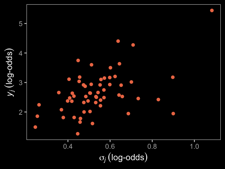
In the estimate column we have all the \(y_j\) values and std.error contains the corresponding \(\sigma_j\) values. Here they are in a plot.

color <- viridis_pal(option = "C")(7)[5]

glms %>% 
  ggplot(aes(x = std.error, y = estimate)) +
  geom_point(color = color) +
  labs(x = expression(sigma[italic(j)]~("log-odds")),
       y = expression(italic(y[j])~("log-odds")))

Fit the Bayesian meta-analysis.

Now are data are ready, we can express our first Bayesian meta-analysis with the formula

\begin{align*} \text{estimate}_j & \sim \operatorname{Normal}(\theta_j, \; \text{std.error}_j) \\ \theta_j & \sim \operatorname{Normal}(\mu, \tau) \\ \mu & \sim \operatorname{Normal}(0, 1.5) \\ \tau & \sim \operatorname{Exponential}(1), \end{align*}

where the last two lines spell out our priors. As we learned in Section 11.1, the \(\operatorname{Normal}(0, 1.5)\) prior in the log-odds space is just about flat on the probability space. If you wanted to be more conservative, consider something like \(\operatorname{Normal}(0, 1)\). Here’s how to fit the model with brms.

me0 <- 
  brm(data = glms, 
      family = gaussian,
      estimate | se(std.error) ~ 1 + (1 | loc),
      prior = c(prior(normal(0, 1.5), class = Intercept),
                prior(exponential(1), class = sd)),
      iter = 2000, warmup = 1000, cores = 4, chains = 4,
      seed = 15)

se() is one of the brms helper functions designed to provide additional information about the criterion variable. Here it informs brm() that each estimate value has an associated measurement error defined in the std.error column. Unlike the mi() function, which we used earlier in the chapter to accommodate measurement error and the Bayesian imputation of missing data, the se() function is specially designed to handle meta-analyses. se() contains a sigma argument which is set to FALSE by default. This will return a model with no estimate for sigma, which is what we want. The uncertainty around the estimate-value for each study \(j\) has already been encoded in the data as std.error.

Let’s look at the model results.

print(me0)

##  Family: gaussian 
##   Links: mu = identity; sigma = identity 
## Formula: estimate | se(std.error) ~ 1 + (1 | loc) 
##    Data: glms (Number of observations: 59) 
##   Draws: 4 chains, each with iter = 2000; warmup = 1000; thin = 1;
##          total post-warmup draws = 4000
## 
## Group-Level Effects: 
## ~loc (Number of levels: 59) 
##               Estimate Est.Error l-95% CI u-95% CI Rhat Bulk_ESS Tail_ESS
## sd(Intercept)     0.43      0.09     0.26     0.61 1.00     1700     2556
## 
## Population-Level Effects: 
##           Estimate Est.Error l-95% CI u-95% CI Rhat Bulk_ESS Tail_ESS
## Intercept     2.55      0.09     2.38     2.72 1.00     2366     2808
## 
## Family Specific Parameters: 
##       Estimate Est.Error l-95% CI u-95% CI Rhat Bulk_ESS Tail_ESS
## sigma     0.00      0.00     0.00     0.00   NA       NA       NA
## 
## Draws were sampled using sampling(NUTS). For each parameter, Bulk_ESS
## and Tail_ESS are effective sample size measures, and Rhat is the potential
## scale reduction factor on split chains (at convergence, Rhat = 1).

Our estimate for heterogeneity across studies, \(\tau\), is about 0.4, suggesting modest differences across the studies. The meta-analytic effect, \(\mu\), is about 2.5. Both, recall, are in the log-odds metric. Here we exponentiate \(\mu\) to get our odds ratio.

fixef(me0) %>% exp()

##           Estimate Est.Error     Q2.5    Q97.5
## Intercept 12.78688  1.091067 10.77015 15.15706

If you look back up to the results reported by Klein and colleagues, you’ll see this is rather close to their OR estimate of 11.54.

Fit the Bayesian muiltilevel alternative.

We said earlier that meta-analysis is just a special case of the multilevel model, applied to summary data. We typically perform meta-analyses on data summaries because historically it has not been the norm among researchers to make their data publicly available. So effect size summaries were the best we typically had for aggregating study results. However, times are changing (e.g., here, here). In this case, Klein and colleagues engaged in open-science practices and reported all their data. Thus we can just directly fit the model

``

where the criterion variable, \(y\), is nested in \(i\) participants within \(j\) locations. The \(\beta\) parameter is analogous to the meta-analytic effect ($\mu$) and \(\sigma_\beta\) is analogous to the expression of heterogeneity in the meta-analytic effect ($\tau$). Here is how to fit the model with brms.

me1 <- 
  brm(data = h, 
      family = binomial,
      y | trials(1) ~ 0 + Intercept + factor + (1 + factor | loc),
      prior = c(prior(normal(0, 1.5), class = b),
                prior(exponential(1), class = sd),
                prior(lkj(2), class = cor)),
      iter = 2000, warmup = 1000, cores = 4, chains = 4,
      seed = 15)

The results for the focal parameters are very similar to those from me0.

print(me1)

##  Family: binomial 
##   Links: mu = logit 
## Formula: y | trials(1) ~ 0 + Intercept + factor + (1 + factor | loc) 
##    Data: h (Number of observations: 6842) 
##   Draws: 4 chains, each with iter = 2000; warmup = 1000; thin = 1;
##          total post-warmup draws = 4000
## 
## Group-Level Effects: 
## ~loc (Number of levels: 59) 
##                                 Estimate Est.Error l-95% CI u-95% CI Rhat Bulk_ESS Tail_ESS
## sd(Intercept)                       0.42      0.07     0.30     0.57 1.00     1593     2426
## sd(factorSideEffect)                0.48      0.09     0.32     0.67 1.00      918     1642
## cor(Intercept,factorSideEffect)    -0.31      0.19    -0.63     0.09 1.01     1014     1909
## 
## Population-Level Effects: 
##                  Estimate Est.Error l-95% CI u-95% CI Rhat Bulk_ESS Tail_ESS
## Intercept           -1.67      0.08    -1.82    -1.53 1.00     1516     1806
## factorSideEffect     2.57      0.09     2.40     2.75 1.00     1509     1846
## 
## Draws were sampled using sampling(NUTS). For each parameter, Bulk_ESS
## and Tail_ESS are effective sample size measures, and Rhat is the potential
## scale reduction factor on split chains (at convergence, Rhat = 1).

Here’s the multilevel version of the effect size as an odds ratio.

fixef(me1)[2, -2] %>% exp()

## Estimate     Q2.5    Q97.5 
## 13.09258 11.01871 15.70430

Here we compare the study specific effect sizes, \(\theta_j\), by our two modeling approaches.

color <- viridis_pal(option = "C")(7)[3]

# how many levels are there?
n_loc <- distinct(h, loc) %>% count() %>% pull(n)

# rank by meta-analysis
ranks <-
  tibble(Estimate = coef(me0)$loc[, 1, "Intercept"],
         index    = 1:n_loc) %>% 
  arrange(Estimate) %>% 
  mutate(rank = 1:n_loc)

rbind(coef(me0)$loc[, , "Intercept"],
      coef(me1)$loc[, , "factorSideEffect"]) %>% 
  data.frame() %>% 
  mutate(index = rep(1:n_loc, times = 2),
         type  = rep(c("meta-analysis", "multilevel model"), each = n_loc)) %>% 
  left_join(select(ranks, -Estimate), 
            by = "index") %>% 
  
  ggplot(aes(x = Estimate, xmin = Q2.5, xmax = Q97.5, y = rank)) +
  geom_pointrange(fatten = 1, color = color) +
  scale_x_continuous(expression(log-odds~effect~size~(theta[italic(j)])), limits = c(0, 4.5)) +
  scale_y_continuous(NULL, breaks = NULL) +
  facet_wrap(~type)

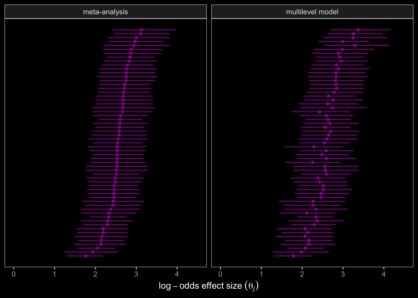
The results are very similar. You might be curious how to show these results in a more conventional looking forest plot where the names of the groups (typically studies) for the \(\theta_j\) values are listed on the left, the point estimate and 95% interval summaries are listed on the right, and the summary for the population level effect, \(\mu\), is listed beneath all all the \(\theta_j\)’s. That’ll require some prep work. First we’ll need to reformat the location names. I’ll save the results in an object called labs.

labs <-
  h %>% 
  mutate(lab = case_when(
    Location == "Social and Work Psychology Department, University of Brasilia, DF, Brazil" ~ "University of Brasilia",
    Location == "Wilfrid Laurier University, Waterloo, Ontario, Canada" ~ "Wilfrid Laurier University",
    Location == "University of British Columbia, Vancouver, Canada" ~ "University of British Columbia",
    Location == "University of Toronto, Scarborough" ~ "University of Toronto",
    Location == "Division of Social Science, The Hong Kong University of Science and Technology, Hong Kong, China" ~ "Hong Kong University of Science and Technology",
    Location == "Chinese Academy of Science, Beijing, China" ~ "Chinese Academy of Science",
    Location == "Shanghai International Studies University, SISU Intercultural Institute, Shanghai, China" ~ "Shanghai International Studies University",
    Location == "Guangdong Literature & Art Vocational College, Guangzhou, China" ~ "Guangdong Literature & Art Vocational College",
    Location == "The University of J. E. Purkyně, Ústí nad Labem, Czech Republic" ~ "The University of J. E. Purkyně",
    Location == "University of Leuven, Belgium" ~ "University of Leuven",
    Location == "Department of Experimental and Applied Psychology, VU Amsterdam, 1081BT, Amsterdam, The Netherlands" ~ "VU Amsterdam",
    Location == "Department of Social Psychology, Tilburg University, P.O. Box 90153, Tilburg, 5000 LE, Netherlands" ~ "Department of Social Psychology, Tilburg University",
    Location == "Eindhoven University of Technology, Eindhoven, Netherlands" ~ "Eindhoven University of Technology",
    Location == "Department of Communication and Information Sciences, P.O. Box 90153, Tilburg, 5000 LE, Netherlands" ~ "Department of Communication and Information Sciences, Tilburg University",
    Location == "University of Navarra, Spain" ~ "University of Navarra",
    Location == "University of Lausanne, Switzerland" ~ "University of Lausanne",
    Location == "Université de Poitiers, France" ~ "Université de Poitiers",
    Location == "Eotvos Lorand University, in Budapest, Hungary" ~ "Eotvos Lorand University",
    Location == "MTurk India Workers" ~ "MTurk India Workers",
    Location == "University of Winchester, Winchester, Hampshire, England" ~ "University of Winchester",
    Location == "Doshisha University, Kyoto, Japan" ~ "Doshisha University",
    Location == "Victoria University of Wellington, New Zealand" ~ "Victoria University of Wellington",
    Location == "University of Social Sciences and Humanities, Wroclaw, Poland" ~ "University of Social Sciences and Humanities",
    Location == "Department of Psychology, SWPS University of Social Sciences and Humanities Campus Sopot, Sopot, Poland" ~ "SWPS University of Social Sciences and Humanities Campus Sopot",
    Location == "badania.net" ~ "badania.net",
    Location == "Universidade do Porto, Portugal" ~ "Universidade do Porto",
    Location == "University of Belgrade, Belgrade, Serbia" ~ "University of Belgrade",
    Location == "University of Johannesburg, Johanneburg, South Africa" ~ "University of Johannesburg",
    Location == "Santiago, Chile" ~ "Santiago, Chile",
    Location == "Universidad de Costa Rica, Costa Rica" ~ "Universidad de Costa Rica",
    Location == "National Autonomous University of Mexico in Mexico City" ~ "National Autonomous University of Mexico",
    Location == "University of the Republic, Montevideo, Uruguay" ~ "University of the Republic",
    Location == "Lund University, Lund, Sweden" ~ "Lund University",
    Location == "Academia Sinica, Taiwan National Taiwan Normal University, Taiwan" ~ "Taiwan National Taiwan Normal University",
    Location == "Bilgi University, Istanbul, Turkey" ~ "Bilgi University",
    Location == "Koç University, Istanbul, Turkey" ~ "Koç University",
    Location == "American University of Sharjah, United Arab Emirates" ~ "American University of Sharjah",
    Location == "University of Hawaii, Honolulu, HI" ~ "University of Hawaii",
    Location == "Social Science and Policy Studies Department, Worcester Polytechnic Institute, Worcester, MA 01609" ~ "Worcester Polytechnic Institute",
    Location == "Department of Psychology, Washington and Lee University, Lexington, VA 24450" ~ "Washington and Lee University",
    Location == "Department of Psychology, San Diego State University, San Diego, CA 92182" ~ "San Diego State University",
    Location == "Tufts" ~ "Tufts",
    Location == "University of Florida, Florida" ~ "University of Florida",
    Location == "University of Illinois at Urbana-Champaign, Champaign, IL" ~ "University of Illinois at Urbana-Champaign",
    Location == "Pacific Lutheran University, Tacoma, WA" ~ "Pacific Lutheran University",
    Location == "University of Virginia, VA" ~ "University of Virginia",
    Location == "Marian University, Indianapolis, IN" ~ "Marian University",
    Location == "Department of Psychology, Ithaca College, Ithaca, NY 14850" ~ "Ithaca College",
    Location == "University of Michigan" ~ "University of Michigan",
    Location == "Department of Psychology, Pennsylvania State University Abington, Abington, PA 19001" ~ "Pennsylvania State University Abington",
    Location == "Department of Psychology, Texas A&M University, College Station, TX 77843" ~ "Texas A&M University",
    Location == "William Paterson University, Wayne, NJ" ~ "William Paterson University",
    Location == "Department of Cognitive Science, Occidental College, Los Angeles, CA" ~ "Occidental College",
    Location == "The Pennsylvania State University" ~ "The Pennsylvania State University",
    Location == "MTurk US Workers" ~ "MTurk US Workers",
    Location == "University of Graz AND the Universty of Vienna" ~ "University of Graz and the Universty of Vienna",
    Location == "University of Potsdam, Germany" ~ "University of Potsdam",
    Location == "Open University of Hong Kong" ~ "Open University of Hong Kong",
    Location == "Concepción, Chile" ~ "Concepción"
  )) %>% 
  distinct(loc, lab)

# what is this?
labs %>% 
  glimpse()

## Rows: 59
## Columns: 2
## $ loc <fct> 1, 2, 3, 4, 5, 6, 7, 8, 9, 10, 11, 12, 13, 14, 15, 16, 17, 18, 19, 20, 21, 22, 23, 24,…
## $ lab <chr> "University of Brasilia", "Wilfrid Laurier University", "University of British Columbi…

Now we’ll do some tricky wrangling with the output from coef() and fixef() to arrange the odds ratio summaries for the population average and the location-specific results.

# this will help us format the labels on the secondary y-axis
my_format <- function(number) {
  formatC(number, digits = 2, format = "f")
}

# grab the theta_j summaries
groups <-
  coef(me1)$loc[, , "factorSideEffect"] %>% 
  data.frame() %>% 
  mutate(loc = distinct(h, loc) %>% pull()) %>% 
  arrange(Estimate)

# grat the mu summary
average <-
  fixef(me1) %>% 
  data.frame() %>% 
  slice(2) %>% 
  mutate(loc = "Average")

# combine and wrangle
draws <-
  bind_rows(groups, average) %>% 
  mutate(rank     = c(1:59, 0),
         Estimate = exp(Estimate),
         Q2.5     = exp(Q2.5),
         Q97.5    = exp(Q97.5)) %>% 
  left_join(labs, by = "loc") %>% 
  arrange(rank) %>% 
  mutate(label   = ifelse(is.na(lab), "POPULATION AVERAGE", lab),
         summary = str_c(my_format(Estimate), " [", my_format(Q2.5), ", ", my_format(Q97.5), "]"))

# what have we done?
draws %>% 
  glimpse()

## Rows: 60
## Columns: 9
## $ Estimate  <dbl> 13.092577, 5.981954, 7.261304, 7.908484, 7.940200, 7.994296, 8.289460, 8.495253,…
## $ Est.Error <dbl> 0.0923085, 0.2430214, 0.3488498, 0.3550866, 0.3343224, 0.2276796, 0.3426444, 0.3…
## $ Q2.5      <dbl> 11.018709, 3.700239, 3.582407, 3.810026, 4.057040, 5.087872, 4.255794, 4.484809,…
## $ Q97.5     <dbl> 15.704304, 9.587316, 14.224359, 15.928584, 15.237924, 12.512837, 16.466681, 15.9…
## $ loc       <chr> "Average", "19", "38", "32", "8", "55", "5", "34", "9", "22", "6", "58", "24", "…
## $ rank      <dbl> 0, 1, 2, 3, 4, 5, 6, 7, 8, 9, 10, 11, 12, 13, 14, 15, 16, 17, 18, 19, 20, 21, 22…
## $ lab       <chr> NA, "MTurk India Workers", "University of Hawaii", "University of the Republic",…
## $ label     <chr> "POPULATION AVERAGE", "MTurk India Workers", "University of Hawaii", "University…
## $ summary   <chr> "13.09 [11.02, 15.70]", "5.98 [3.70, 9.59]", "7.26 [3.58, 14.22]", "7.91 [3.81, …

Here’s our custom forest plot.

draws %>% 
  ggplot(aes(x = Estimate, xmin = Q2.5, xmax = Q97.5, y = rank)) +
  geom_interval(aes(color = label == "POPULATION AVERAGE"),
                size = 1/2) +
  geom_point(aes(size = 1 - Est.Error, color = label == "POPULATION AVERAGE"),
             shape = 15) +
  scale_color_viridis_d(option = "C", begin = .33, end = .67) +
  scale_size_continuous(range = c(1, 3.5)) +
  scale_x_continuous("odds ratio", breaks = 1:6 * 10, expand = expansion(mult = c(0.005, 0.005))) +
  scale_y_continuous(NULL, breaks = 0:59, limits = c(-1, 60), expand = c(0, 0),
                     labels = pull(draws, label),
                     sec.axis = dup_axis(labels = pull(draws, summary))) +
  theme(text = element_text(family = "Times"),
        axis.text.y = element_text(hjust = 0, color = "white", size = 7),
        axis.text.y.right = element_text(hjust = 1, size = 7),
        axis.ticks.y = element_blank(),
        panel.background = element_rect(fill = "grey8"),
        panel.border = element_rect(color = "transparent"))

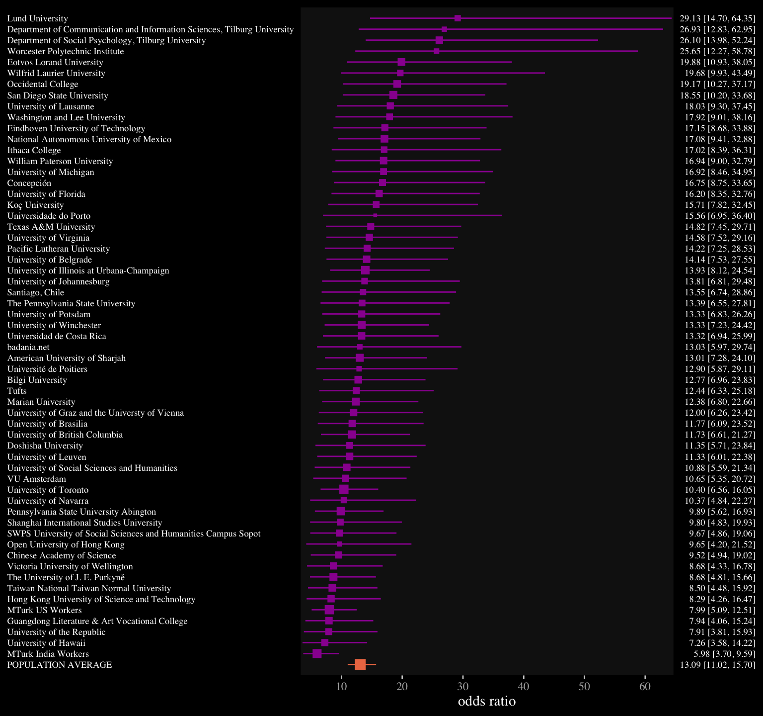
You may have noticed this plot is based on the results of our multilevel model, me1. We could have done the same basic thing with the results from the more conventional meta-analysis model, me0, too.

I’m not aware this it typical in random effect meta-analyses, but it might be useful to further clarify the meaning of the two primary parameters, \(\mu\) and \(\tau\). Like with the forest plot, above, we could examine these with either me0 or me1. For kicks, we’ll use me0 (the conventional Bayesian meta-analysis). In the output from as_draws_df(me0), \(\mu\) and \(\tau\) are in the columns named b_Intercept and sd_loc__Intercept, respectively.

draws <- as_draws_df(me0)

draws %>% 
  select(b_Intercept:sd_loc__Intercept) %>% 
  head()

## # A tibble: 6 × 2
##   b_Intercept sd_loc__Intercept
##         <dbl>             <dbl>
## 1        2.53             0.442
## 2        2.50             0.369
## 3        2.68             0.424
## 4        2.50             0.310
## 5        2.48             0.366
## 6        2.61             0.544

If you scroll back above, you’ll see our random effect meta-analysis explicitly presumed our empirical effect-size estimates \(y_j\) are approximations of the true effect sizes \(\theta_j\), which are themselves normally distributed in the population of possible effect sizes from similar studies: \(\theta_j \sim \operatorname{Normal}(\mu, \tau)\). Why not use our posterior samples to simulate draws from \(\operatorname{Normal}(\mu, \tau)\) to get a sense of what this distribution might look like? Recall that the parameters are in the log-odds metric. We’ll present the distribution in that metric and as odds ratios.

color <- viridis_pal(option = "C")(7)[6]
set.seed(15)

draws %>% 
  transmute(lo = rnorm(n(), mean = b_Intercept, sd = sd_loc__Intercept),
            or = rnorm(n(), mean = b_Intercept, sd = sd_loc__Intercept) %>% exp()) %>% 
  slice(1:1e3) %>% 
  pivot_longer(lo:or, values_to = "effect size") %>% 
  mutate(name = factor(name, labels = c("log-odds", "odds ratio"))) %>% 
  
  ggplot(aes(x = `effect size`, y = 0)) +
  geom_dots(color = color, fill = color) +
  scale_y_continuous(NULL, breaks = NULL) +
  xlab(expression(Normal(mu*', '*tau))) +
  theme(text = element_text(family = "Times"),
        strip.background = element_rect(color = "transparent")) +
  facet_wrap(~name, scales = "free")

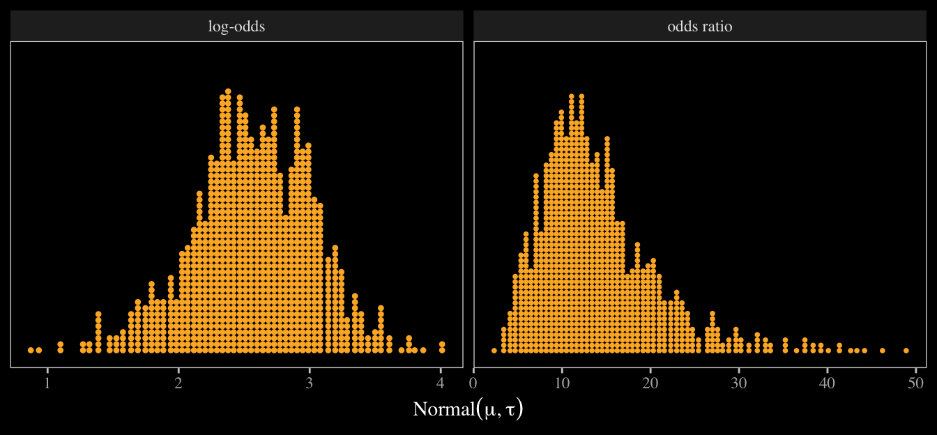
Both panels show 1,000 draws, each of which is depicted by a single dot. If we were to run this experiment 1,000 times and compute the effect size separately for each one, this is what we’d expect those distributions of effect sizes to look like. Seems like there’s a lot of variation in there, eh? The next time you observe your fellow scientists debating over whether a study replicated or not, keep these distributions in mind. Once you start thinking about distributions, replication becomes a tricky notion.

Parting thoughts.

There are other things you might do with these data. For example, you might inspect how much the effect size varies between those from WEIRD and non-WEIRD countries. You might also model the data as clustered by Language rather than by Location. But I think we’ve gone far enough to get you started.

If you’d like to learn more about these methods, do check out Vourre’s Meta-analysis is a special case of Bayesian multilevel modeling. You might also read Williams, Rast, and Bürkner’s ( 2018) manuscript, Bayesian meta-analysis with weakly informative prior distributions. For an alternative workflow, consider the baggr package ( Wiecek & Meager, 2022), which is designed to fit hierarchical Bayesian meta-analyses with Stan under the hood.

Session info

sessionInfo()

## R version 4.2.0 (2022-04-22)
## Platform: x86_64-apple-darwin17.0 (64-bit)
## Running under: macOS Big Sur/Monterey 10.16
## 
## Matrix products: default
## BLAS:   /Library/Frameworks/R.framework/Versions/4.2/Resources/lib/libRblas.0.dylib
## LAPACK: /Library/Frameworks/R.framework/Versions/4.2/Resources/lib/libRlapack.dylib
## 
## locale:
## [1] en_US.UTF-8/en_US.UTF-8/en_US.UTF-8/C/en_US.UTF-8/en_US.UTF-8
## 
## attached base packages:
## [1] stats     graphics  grDevices utils     datasets  methods   base     
## 
## other attached packages:
##  [1] tidybayes_3.0.2   broom_1.0.1       viridis_0.6.2     viridisLite_0.4.1 ggdark_0.2.1     
##  [6] brms_2.18.0       Rcpp_1.0.9        forcats_0.5.1     stringr_1.4.1     dplyr_1.0.10     
## [11] purrr_0.3.4       readr_2.1.2       tidyr_1.2.1       tibble_3.1.8      ggplot2_3.4.0    
## [16] tidyverse_1.3.2  
## 
## loaded via a namespace (and not attached):
##   [1] readxl_1.4.1         backports_1.4.1      plyr_1.8.7           igraph_1.3.4        
##   [5] svUnit_1.0.6         splines_4.2.0        crosstalk_1.2.0      TH.data_1.1-1       
##   [9] rstantools_2.2.0     inline_0.3.19        digest_0.6.30        htmltools_0.5.3     
##  [13] fansi_1.0.3          magrittr_2.0.3       checkmate_2.1.0      googlesheets4_1.0.1 
##  [17] tzdb_0.3.0           modelr_0.1.8         RcppParallel_5.1.5   matrixStats_0.62.0  
##  [21] vroom_1.5.7          xts_0.12.1           sandwich_3.0-2       prettyunits_1.1.1   
##  [25] colorspace_2.0-3     rvest_1.0.2          ggdist_3.2.0         haven_2.5.1         
##  [29] xfun_0.35            callr_3.7.3          crayon_1.5.2         jsonlite_1.8.3      
##  [33] lme4_1.1-31          survival_3.4-0       zoo_1.8-10           glue_1.6.2          
##  [37] gtable_0.3.1         gargle_1.2.0         emmeans_1.8.0        distributional_0.3.1
##  [41] pkgbuild_1.3.1       rstan_2.21.7         abind_1.4-5          scales_1.2.1        
##  [45] mvtnorm_1.1-3        DBI_1.1.3            miniUI_0.1.1.1       xtable_1.8-4        
##  [49] bit_4.0.4            stats4_4.2.0         StanHeaders_2.21.0-7 DT_0.24             
##  [53] htmlwidgets_1.5.4    httr_1.4.4           threejs_0.3.3        arrayhelpers_1.1-0  
##  [57] posterior_1.3.1      ellipsis_0.3.2       pkgconfig_2.0.3      loo_2.5.1           
##  [61] farver_2.1.1         sass_0.4.2           dbplyr_2.2.1         utf8_1.2.2          
##  [65] labeling_0.4.2       tidyselect_1.1.2     rlang_1.0.6          reshape2_1.4.4      
##  [69] later_1.3.0          munsell_0.5.0        cellranger_1.1.0     tools_4.2.0         
##  [73] cachem_1.0.6         cli_3.4.1            generics_0.1.3       ggridges_0.5.3      
##  [77] evaluate_0.18        fastmap_1.1.0        yaml_2.3.5           bit64_4.0.5         
##  [81] processx_3.8.0       knitr_1.40           fs_1.5.2             nlme_3.1-159        
##  [85] mime_0.12            projpred_2.2.1       xml2_1.3.3           compiler_4.2.0      
##  [89] bayesplot_1.9.0      shinythemes_1.2.0    rstudioapi_0.13      curl_4.3.2          
##  [93] gamm4_0.2-6          reprex_2.0.2         bslib_0.4.0          stringi_1.7.8       
##  [97] highr_0.9            ps_1.7.2             blogdown_1.15        Brobdingnag_1.2-8   
## [101] lattice_0.20-45      Matrix_1.4-1         nloptr_2.0.3         markdown_1.1        
## [105] shinyjs_2.1.0        tensorA_0.36.2       vctrs_0.5.0          pillar_1.8.1        
## [109] lifecycle_1.0.3      jquerylib_0.1.4      bridgesampling_1.1-2 estimability_1.4.1  
## [113] httpuv_1.6.5         R6_2.5.1             bookdown_0.28        promises_1.2.0.1    
## [117] gridExtra_2.3        codetools_0.2-18     boot_1.3-28          colourpicker_1.1.1  
## [121] MASS_7.3-58.1        gtools_3.9.3         assertthat_0.2.1     withr_2.5.0         
## [125] shinystan_2.6.0      multcomp_1.4-20      mgcv_1.8-40          parallel_4.2.0      
## [129] hms_1.1.1            grid_4.2.0           coda_0.19-4          minqa_1.2.5         
## [133] rmarkdown_2.16       googledrive_2.0.0    shiny_1.7.2          lubridate_1.8.0     
## [137] base64enc_0.1-3      dygraphs_1.1.1.6

References

Gelman, A., Carlin, J. B., Stern, H. S., Dunson, D. B., Vehtari, A., & Rubin, D. B. (2013). Bayesian data analysis (Third Edition). CRC press. https://stat.columbia.edu/~gelman/book/
Hauser, M., Cushman, F., Young, L., Jin, R. K.-X., & Mikhail, J. (2007). A dissociation between moral judgments and justifications. Mind & Language, 22(1), 1–21. https://doi.org/10.1111/j.1468-0017.2006.00297.x
Klein, R. A., Vianello, M., Hasselman, F., Adams, B. G., Adams, R. B., Alper, S., Aveyard, M., Axt, J. R., Babalola, M. T., Bahník, Š., Batra, R., Berkics, M., Bernstein, M. J., Berry, D. R., Bialobrzeska, O., Binan, E. D., Bocian, K., Brandt, M. J., Busching, R., … Nosek, B. A. (2018). Many Labs 2: Investigating variation in replicability across samples and settings. Advances in Methods and Practices in Psychological Science, 1(4), 443–490. https://doi.org/10.1177/2515245918810225
Kurz, A. S. (2020a). Statistical rethinking with brms, Ggplot2, and the tidyverse: Second edition (version 0.1.1). https://bookdown.org/content/4857/
Kurz, A. S. (2020b). Statistical rethinking with brms, ggplot2, and the tidyverse (version 1.2.0). https://doi.org/10.5281/zenodo.3693202
McElreath, R. (2015). Statistical rethinking: A Bayesian course with examples in R and Stan. CRC press. https://xcelab.net/rm/statistical-rethinking/
McElreath, R. (2020). Statistical rethinking: A Bayesian course with examples in R and Stan (Second Edition). CRC Press. https://xcelab.net/rm/statistical-rethinking/
Wiecek, W., & Meager, R. (2022). baggr: Bayesian aggregate treatment effects [Manual]. https://CRAN.R-project.org/package=baggr
Williams, D. R., Rast, P., & Bürkner, P.-C. (2018). Bayesian meta-analysis with weakly informative prior distributions. https://doi.org/10.31234/osf.io/7tbrm
- Posted on:
- October 16, 2020
- Length:
- 30 minute read, 6207 words