Got overdispersion? Try observation-level random effects with the Poisson-lognormal mixture

Version 1.1.0

Edited on December 12, 2022, to use the new as_draws_df() workflow.

What?

One of Tristan Mahr’s recent Twitter threads almost broke my brain.

wait when people talk about treating overdispersion by using random effects, they sometimes put a random intercept on each row?? https://t.co/7NjG4uw3nz pic.twitter.com/fo8Ylcejqv

— guy whose whole personality is duckdb 🦆 (@tjmahr) July 8, 2021

It turns out that you can use random effects on cross-sectional count data. Yes, that’s right. Each count gets its own random effect. Some people call this observation-level random effects and it can be a tricky way to handle overdispersion. The purpose of this post is to show how to do this and to try to make sense of what it even means.

Background

First, I should clarify a bit. Mahr’s initial post and much of the thread to follow primarily focused on counts within the context of binomial data. If you’ve ever read a book on the generalized linear model (GLM), you know that the two broad frameworks for modeling counts are as binomial or Poisson. The basic difference is if your counts are out of a known number of trials (e.g., I got 3 out of 5 questions correct in my pop quiz, last week¹), the binomial is generally the way to go. However, if your counts aren’t out of a well-defined total (e.g., I drank 1497 cups of coffee², last year), the Poisson distribution offers a great way to think about your data. In this post, we’ll be focusing on Poisson-like counts.

The Poisson distribution is named after the French mathematician Siméon Denis Poisson, who lived and died about 200 years ago. Poisson’s distribution is valid for non-negative integers, which is basically what counts are. The distribution has just one parameter, \(\lambda\), which controls both its mean and variance and imposes the assumption that the mean of your counts is the same as the variance. On the one hand, this is great because it keeps things simple–parsimony and all. On the other hand, holding the mean and variance the same is a really restrictive assumption and it just doesn’t match up well with a lot of real-world data.

This Poisson assumption that the mean equals the variance is sometimes called equidispersion. Count data violate the equidispersion assumption when their variance is smaller than their mean (underdispersion) or when their variance is larger than their mean (overdispersion). In practice, overdispersion tends to crop up most often. Real-world count data are overdispersed so often that statisticians have had to come up with a mess of strategies to handle the problem. In the applied statistics that I’m familiar with, the two most common ways to handle overdispersed count data are with the negative-binomial model, or with random effects. We’ll briefly cover both.

Negative-binomial counts.

As its name implies, the negative-binomial model has a deep relationship with the binomial model. I’m not going to go into those details, but Hilbe covered them in his well-named ( 2011) textbook, if you’re curious. Basically, the negative-binomial model adds a dispersion parameter to the Poisson. Different authors refer to it with different names. Hilbe, for example, called it both \(r\) and \(\nu\). Bürkner ( 2021b) and the Stan Development Team ( 2021) both call it \(\phi\). By which ever name, the negative-binomial overdispersion parameter helps disentangle the mean from the variance in a set of counts. The way it does it is by re-expressing the count data as coming from a mixture where each count is from its own Poisson distribution with its own \(\lambda\) parameter. Importantly, the \(\lambda\)’s in this mixture of Poissons follow a gamma distribution, which is why the negative binomial is also sometimes referred to as a gamma-Poisson model. McElreath ( 2020), for example, generally prefers to speak in terms of the gamma-Poisson.

Poission counts with random intercepts.

Another way to handle overdispersion is to ask whether the data are grouped. In my field, this naturally occurs when you collect longitudinal data. My counts, over time, will differ form your counts, over time, and we accommodate that by adding a multilevel structure to the model. This, then, takes us to the generalized linear mixed model (GLMM), which is covered in text books like Cameron & Trivedi ( 2013); Gelman & Hill ( 2006); and McElreath ( 2020). Say your data have \(J\) groups. With a simple random-intercept Poisson model, each group of counts gets its own \(\lambda_j\) parameter and the population of those \(\lambda_j\)’s is described in terms of a grand mean (an overall \(\lambda\) intercept) and variation around that grand mean (typically a standard deviation or variance parameter). Thus, if your \(y\) data are counts from \(I\) cases clustered within \(J\) groups, the random-intercept Poisson model can be expressed as

$$ \begin{align*} y_{ij} & \sim \operatorname{Poisson}(\lambda_{ij}) \\ \log(\lambda_{ij}) & = \beta_0 + \zeta_{0j} \\ \zeta_{0j} & \sim \operatorname{Normal}(0, \sigma_0) \end{align*} $$

where the grand mean is \(\beta_0\), the group-specific deviations around the grand mean are the \(\zeta_{0j}\)’s, and the variation across those \(\zeta_{0j}\)’s is expressed by a standard-deviation parameter \(\sigma_0\). Thus following the typical GLMM convention, we model the group-level deviations with the normal distribution. Also notice that whether we’re talking about single-level GLMs or multilevel GLMMs, we typically model \(\log \lambda\), instead of \(\lambda\). This prevents the model from predicting negative counts. Keep this in mind.

Anyway, the random-intercept Poisson model can go a long way for handling overdispersion when your data are grouped. It’s also possible to combine this approach with the last one and fit a negative-binomial model with a random intercept, too. Though I haven’t seen this used much in practice, you can even take a distributional model approach ( Bürkner, 2021a) and set the negative-binomial dispersion parameter to random, too. That, for example, could look like

$$ \begin{align*} y_{ij} & \sim \operatorname{Gamma-Poisson}(\lambda_{ij}, \phi_{ij}) \\ \log(\lambda_{ij}) & = \beta_0 + \zeta_{0j} \\ \log(\phi_{ij}) & = \gamma_0 + \zeta_{1j} \\ \zeta_{0j} & \sim \operatorname{Normal}(0, \sigma_0) \\ \zeta_{1j} & \sim \operatorname{Normal}(0, \sigma_1). \end{align*} $$

There’s a third option: The Poisson-lognormal.

Now a typical condition for a random-intercept model (whether using the Poison, the negative-binomial, or any other likelihood function) is that at least some of the \(J\) groups, if not most or all, contain two or more cases. For example, in a randomized controlled trial you might measure the outcome variable 3 or 5 or 10 times over the course of the trial. In a typical non-experimental experience-sampling study, you might get 10 or 50 or a few hundred measurements from each participant over the course of a few days, weeks, or months. Either way, we tend to have multiple \(I\)’s within each level of \(J\). As it turns out, you don’t have to restrict yourself that way. With the observation-level random effects (OLRE) approach, each case (each level of \(I\)) gets its own random effect (see Harrison, 2014).

But why would you do that?

Think back to the conventional regression model where some variable \(x\) is predicting some continuous variable \(y\). We can express the model as

$$ \begin{align*} y_i & \sim \operatorname{Normal}(\mu_i, \sigma) \\ \mu_i & = \beta_0 + \beta_1 x_i, \end{align*} $$

where the residual variance not accounted for by \(x\) is captured in \(\sigma\)³. Thus \(\sigma\) can be seen as a residual-variance term. The conventional Poisson model,

$$ \begin{align*} y_i & \sim \operatorname{Poisson}(\lambda_i) \\ \log(\lambda_i) & = \beta_0 + \beta_1 x_i, \end{align*} $$

doesn’t have a residual-variance term. Rather, the variance in the data is deterministically controlled by the linear model on \(\log(\lambda_i)\), which works great in the case of equidispersion, but fails when the data are overdispersed. Hence the negative-binomial and the random-intercept models. But what if we could tack on a residual variance term? It might take on a form like

$$ \begin{align*} y_i & \sim \operatorname{Poisson}(\lambda_i) \\ \log(\lambda_i) & = \beta_0 + \beta_1 x_i + \epsilon_i, \end{align*} $$

where \(\epsilon_i\) is the residual variation in \(y_i\) not captured by the deterministic part of the linear model for \(\log(\lambda_i)\). Following the conventional regression model, we might make our lives simple and further presume \(\epsilon_i \sim \operatorname{Normal}(0, \sigma_\epsilon)\). Though he didn’t use this style of notation, that’s basically the insight from Bulmer ( 1974). But rather than speak in terms of \(\epsilon_i\) and residual variance, Bulmer proposed an alternative to the gamma-Poisson mixture and asked his audience to imagine each count in the data was from its own Poisson distribution with its own \(\lambda\) parameter, but that those \(\lambda\) parameters were distributed according to the lognormal distribution. Now Bulmer had a substantive motivation for proposing the lognormal based on the species-abundance data and I’m not going to get into any of that. But the basic point was, if we can have a gamma-distributed mixture of \(\lambda\)’s, why not a lognormal mixture, instead?

The trouble with Bulmer’s lognormal-mixture approach is it’s not readily available in most software packages. However, notice what happens when you specify an OLRE model with the Poisson likelihood:

$$ \begin{align*} y_i & \sim \operatorname{Poisson}(\lambda_i) \\ \log(\lambda_i) & = \beta_0 + \zeta_{0i} \\ \zeta_{0i} & \sim \operatorname{Normal}(0, \sigma_0). \end{align*} $$

In this case, \(\zeta_{0i}\) now looks a lot like the \(\epsilon_i\) term in a standard intercepts-only regression model. Further, since the linear model is defined for \(\log(\lambda_i)\), that means the \(\zeta_{0i}\) terms will be log-normally distributed in the exponentiated \(\log(\lambda_i)\) space. In essence, the OLRE-Poisson model is a way to hack your multilevel regression software to fit a Poisson-lognormal model for overdispersed counts.

Now we have a sense of the theory, it’s time to fit some models.

Empirical example: Salamander data

We need data.

As per usual, we’ll be working within R ( R Core Team, 2022). We’ll be fitting our models with brms ( Bürkner, 2017, 2018, 2022) and most of our data wrangling and plotting work will be done with aid from the tidyverse ( Wickham et al., 2019; Wickham, 2022) and friends–patchwork ( Pedersen, 2022) and tidybayes ( Kay, 2022). We’ll take our data set from McElreath’s ( 2020) rethinking package.

library(brms)
library(tidyverse)
library(tidybayes)
library(patchwork)

data(salamanders, package = "rethinking")

glimpse(salamanders)

## Rows: 47
## Columns: 4
## $ SITE      <int> 1, 2, 3, 4, 5, 6, 7, 8, 9, 10, 11, 12, 13, 14, 15, 16, 17, 1…
## $ SALAMAN   <int> 13, 11, 11, 9, 8, 7, 6, 6, 5, 5, 4, 3, 3, 3, 3, 3, 2, 2, 2, …
## $ PCTCOVER  <int> 85, 86, 90, 88, 89, 83, 83, 91, 88, 90, 87, 83, 87, 89, 92, …
## $ FORESTAGE <int> 316, 88, 548, 64, 43, 368, 200, 71, 42, 551, 675, 217, 212, …

The data are in the salamanders data frame, which contains counts of salamanders from 47 locations in northern California ( Welsh Jr & Lind, 1995). Our count variable is SALAMAN. The location for each count is indexed by the SITE column. You could use the other two variables as covariates, but we won’t be focusing on those in this post. Here’s what SALAMAN looks like.

# adjust the global plotting theme
theme_set(theme_classic())

salamanders %>% 
  ggplot(aes(x = SALAMAN)) +
  geom_bar()

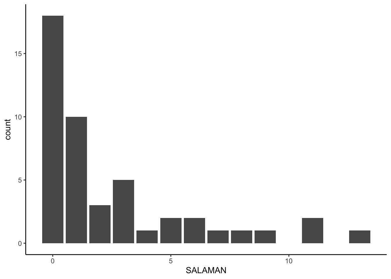
Those data look overdispersed. We can get a quick sense of the overdispersion with sample statistics.

salamanders %>% 
  summarise(mean = mean(SALAMAN),
            variance = var(SALAMAN)) 

##       mean variance
## 1 2.468085 11.38483

For small-$N$ data, we shouldn’t expect the mean to be exactly the same as the variance in Poisson data. This big of a difference, though, suggests⁴ overdispersion even with a modest \(N = 47\).

Fit the models.

We’ll fit three intercepts-only models. The first will be a conventional Poisson model and the second will be the negative binomial (a.k.a. the gamma-Poisson mixture). We’ll finish off with our Poisson-lognormal mixture via the OLRE technique. Since we’re working with Bayesian software, we’ll need priors. Though I’m not going to explain them in any detail, we’ll be using the weakly-regularizing approach advocated for in McElreath ( 2020).

Here’s how to fit the models with brms.

# conventional Poisson
fit1 <-
  brm(data = salamanders, 
      family = poisson,
      SALAMAN ~ 1,
      prior(normal(log(3), 0.5), class = Intercept),
      cores = 4, seed = 1)

# gamma-Poisson mixture
fit2 <-
  brm(data = salamanders, 
      family = negbinomial,
      SALAMAN ~ 1,
      prior = c(prior(normal(log(3), 0.5), class = Intercept),
                prior(gamma(0.01, 0.01), class = shape)),
      cores = 4, seed = 1)

# Poisson-lognormal mixture
fit3 <-
  brm(data = salamanders, 
      family = poisson,
      SALAMAN ~ 1 + (1 | SITE),
      prior = c(prior(normal(log(3), 0.5), class = Intercept),
                prior(exponential(1), class = sd)),
      cores = 4, seed = 1)

Evaluate the models.

Here’s a quick parameter summary for each of the models.

print(fit1)

##  Family: poisson 
##   Links: mu = log 
## Formula: SALAMAN ~ 1 
##    Data: salamanders (Number of observations: 47) 
##   Draws: 4 chains, each with iter = 2000; warmup = 1000; thin = 1;
##          total post-warmup draws = 4000
## 
## Population-Level Effects: 
##           Estimate Est.Error l-95% CI u-95% CI Rhat Bulk_ESS Tail_ESS
## Intercept     0.91      0.09     0.73     1.08 1.00     1483     1967
## 
## Draws were sampled using sampling(NUTS). For each parameter, Bulk_ESS
## and Tail_ESS are effective sample size measures, and Rhat is the potential
## scale reduction factor on split chains (at convergence, Rhat = 1).

print(fit2)

##  Family: negbinomial 
##   Links: mu = log; shape = identity 
## Formula: SALAMAN ~ 1 
##    Data: salamanders (Number of observations: 47) 
##   Draws: 4 chains, each with iter = 2000; warmup = 1000; thin = 1;
##          total post-warmup draws = 4000
## 
## Population-Level Effects: 
##           Estimate Est.Error l-95% CI u-95% CI Rhat Bulk_ESS Tail_ESS
## Intercept     0.95      0.21     0.54     1.36 1.00     2908     2195
## 
## Family Specific Parameters: 
##       Estimate Est.Error l-95% CI u-95% CI Rhat Bulk_ESS Tail_ESS
## shape     0.58      0.18     0.30     1.01 1.00     3607     2640
## 
## Draws were sampled using sampling(NUTS). For each parameter, Bulk_ESS
## and Tail_ESS are effective sample size measures, and Rhat is the potential
## scale reduction factor on split chains (at convergence, Rhat = 1).

print(fit3)

##  Family: poisson 
##   Links: mu = log 
## Formula: SALAMAN ~ 1 + (1 | SITE) 
##    Data: salamanders (Number of observations: 47) 
##   Draws: 4 chains, each with iter = 2000; warmup = 1000; thin = 1;
##          total post-warmup draws = 4000
## 
## Group-Level Effects: 
## ~SITE (Number of levels: 47) 
##               Estimate Est.Error l-95% CI u-95% CI Rhat Bulk_ESS Tail_ESS
## sd(Intercept)     1.28      0.23     0.89     1.80 1.00     1117     1435
## 
## Population-Level Effects: 
##           Estimate Est.Error l-95% CI u-95% CI Rhat Bulk_ESS Tail_ESS
## Intercept     0.34      0.22    -0.12     0.75 1.00     1687     2533
## 
## Draws were sampled using sampling(NUTS). For each parameter, Bulk_ESS
## and Tail_ESS are effective sample size measures, and Rhat is the potential
## scale reduction factor on split chains (at convergence, Rhat = 1).

We might use the pp_check() function to get a graphic sense of how well each model fit the data.

p1 <-
  pp_check(fit1, type = "bars", nsample = 150, fatten = 1, size = 1/2) +
  scale_y_continuous(NULL, breaks = NULL) +
  coord_cartesian(xlim = c(0, 15),
                  ylim = c(0, 26)) +
  labs(title = "fit1",
       subtitle = "Conventional Poisson")

p2 <-
  pp_check(fit2, type = "bars", nsample = 150, fatten = 1, size = 1/2) +
  scale_y_continuous(NULL, breaks = NULL) +
  coord_cartesian(xlim = c(0, 15),
                  ylim = c(0, 26)) +
  labs(title = "fit2",
       subtitle = "Gamma-Poisson mixture")

p3 <-
  pp_check(fit3, type = "bars", nsample = 150, fatten = 1, size = 1/2) +
  scale_y_continuous(NULL, breaks = NULL) +
  coord_cartesian(xlim = c(0, 15),
                  ylim = c(0, 26)) +
  labs(title = "fit3",
       subtitle = "Poisson-lognormal mixture")

p1 + p2 + p3 + plot_layout(guides = "collect")

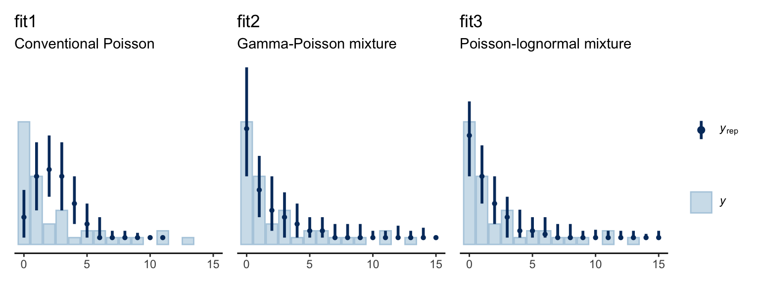
The conventional Poisson model seems like a disaster. Both the gamma-Poisson and the Poisson-lognormal models seemed to capture the data much better. We also might want to compare the models with information criteria. Here we’ll use the LOO.

fit1 <- add_criterion(fit1, criterion = "loo")
fit2 <- add_criterion(fit2, criterion = "loo")
fit3 <- add_criterion(fit3, criterion = "loo")

When I first executed that code, I got the following warning message:

Found 29 observations with a pareto_k > 0.7 in model ‘fit3’. It is recommended to set ‘moment_match = TRUE’ in order to perform moment matching for problematic observations.

To use the moment_match = TRUE option within the add_criterion() function, you have to specify save_pars = save_pars(all = TRUE) within brm() when fitting the model. Here’s how to do that.

# fit the Poisson-lognormal mixture, again
fit3 <-
  brm(data = salamanders, 
      family = poisson,
      SALAMAN ~ 1 + (1 | SITE),
      prior = c(prior(normal(log(3), 0.5), class = Intercept),
                prior(exponential(1), class = sd)),
      cores = 4, seed = 1,
      # here's the new part
      save_pars = save_pars(all = TRUE))

# add the LOO
fit3 <- add_criterion(
  fit3, criterion = "loo", 
  # this part is new, too
  moment_match = TRUE
)

Now we’re ready to compare the models with the LOO.

loo_compare(fit1, fit2, fit3, criterion = "loo") %>% 
  print(simplify = F)

##      elpd_diff se_diff elpd_loo se_elpd_loo p_loo  se_p_loo looic  se_looic
## fit3    0.0       0.0   -89.8      6.6        20.2    1.4    179.6   13.2  
## fit2   -8.2       2.3   -98.0      8.3         1.6    0.2    196.0   16.6  
## fit1  -50.5      13.9  -140.4     17.4         4.3    1.2    280.7   34.8

Even after accounting for model complexity, the Poisson-lognormal model appears to be the best fit for the data. Next we consider how, exactly, does one interprets the parameters of the Poisson-lognormal model.

How does one interpret the Poisson-lognormal model?

A nice quality of both the conventional Poisson model and the gamma-Poisson model is the intercept for each corresponds directly with the mean of the original data, after exponentiation. The mean of the SALAMAN variable, recall, was 2.5. Here are the summaries for their exponentiated intercepts.

# conventional Poisson
fixef(fit1)[, -2] %>% exp() %>% round(digits = 2)

## Estimate     Q2.5    Q97.5 
##     2.48     2.06     2.94

# gamma-Poisson
fixef(fit2)[, -2] %>% exp() %>% round(digits = 2)

## Estimate     Q2.5    Q97.5 
##     2.58     1.72     3.89

Both are really close to the sample mean. Here’s the exponentiated intercept for the Poisson-lognormal model.

fixef(fit3)[, -2] %>% exp() %>% round(digits = 2)

## Estimate     Q2.5    Q97.5 
##     1.40     0.89     2.12

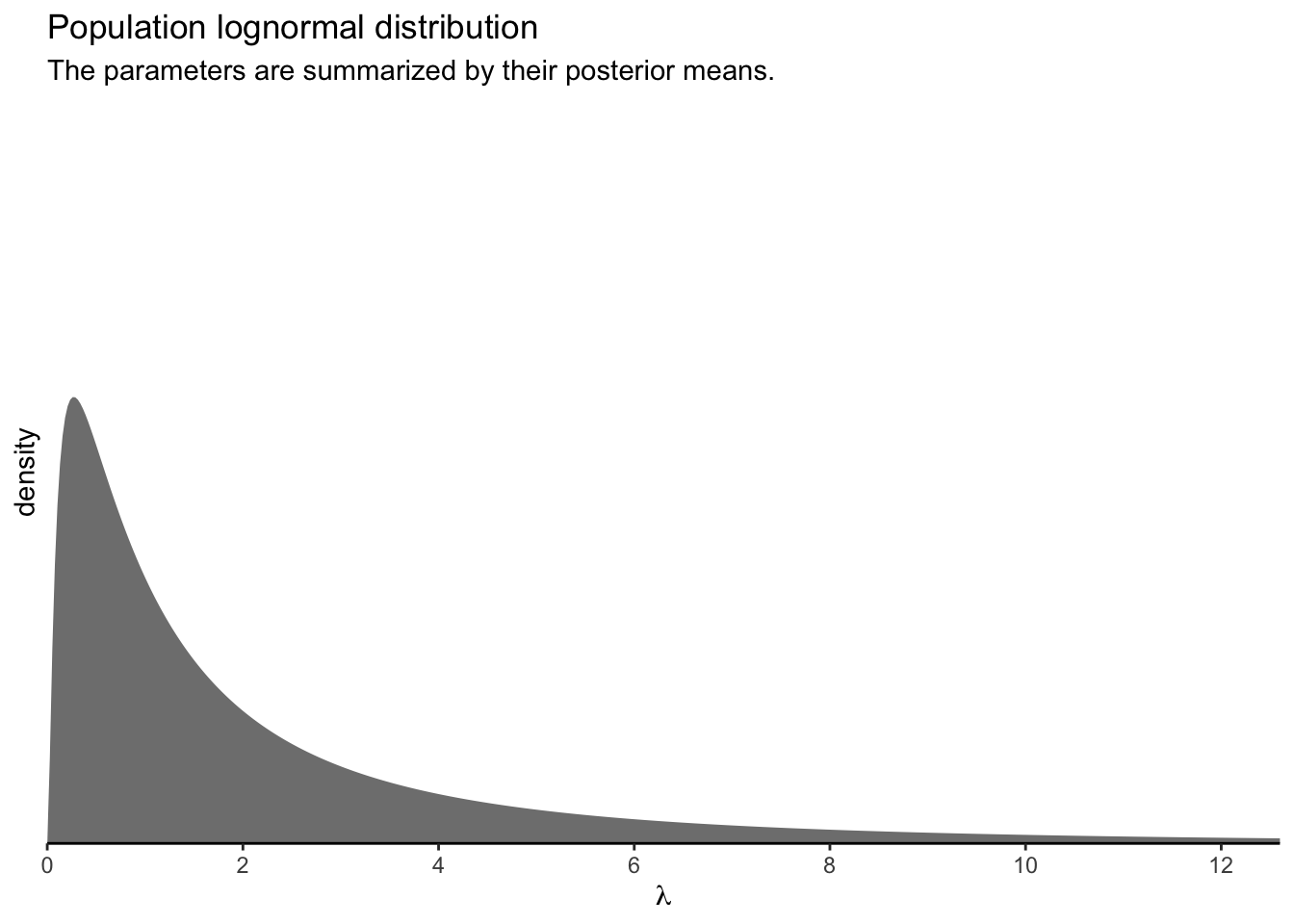
Wow, that’s not even close! What gives? Well, keep in mind that with the OLRE Poisson-lognormal model, the intercept is the \(\mu\) parameter for the lognormal distribution of \(\lambda\) parameters. In a similar way, the level-2 standard deviation (execute posterior_summary(fit3)["sd_SITE__Intercept", ]) is the \(\sigma\) parameter for that lognormal distribution. Keeping things simple, for the moment, here’s what that lognormal distribution looks like if we take the posterior means for those parameters and insert them into the parameter arguments of the dlnorm() function.

p1 <-
  tibble(lambda = seq(from = 0, to = 13, length.out = 500)) %>% 
  mutate(d = dlnorm(lambda, 
                    meanlog = posterior_summary(fit3)[1, 1], 
                    sdlog = posterior_summary(fit3)[2, 1])) %>% 
  
  ggplot(aes(x = lambda, y = d)) +
  geom_area(fill = "grey50") +
  scale_x_continuous(expression(lambda), breaks = 0:6 * 2, 
                     expand = expansion(mult = c(0, 0.05))) +
  scale_y_continuous("density", breaks = NULL, 
                     expand = expansion(mult = c(0, 0.05))) +
  coord_cartesian(xlim = c(0, 12),
                  ylim = c(0, 0.8)) +
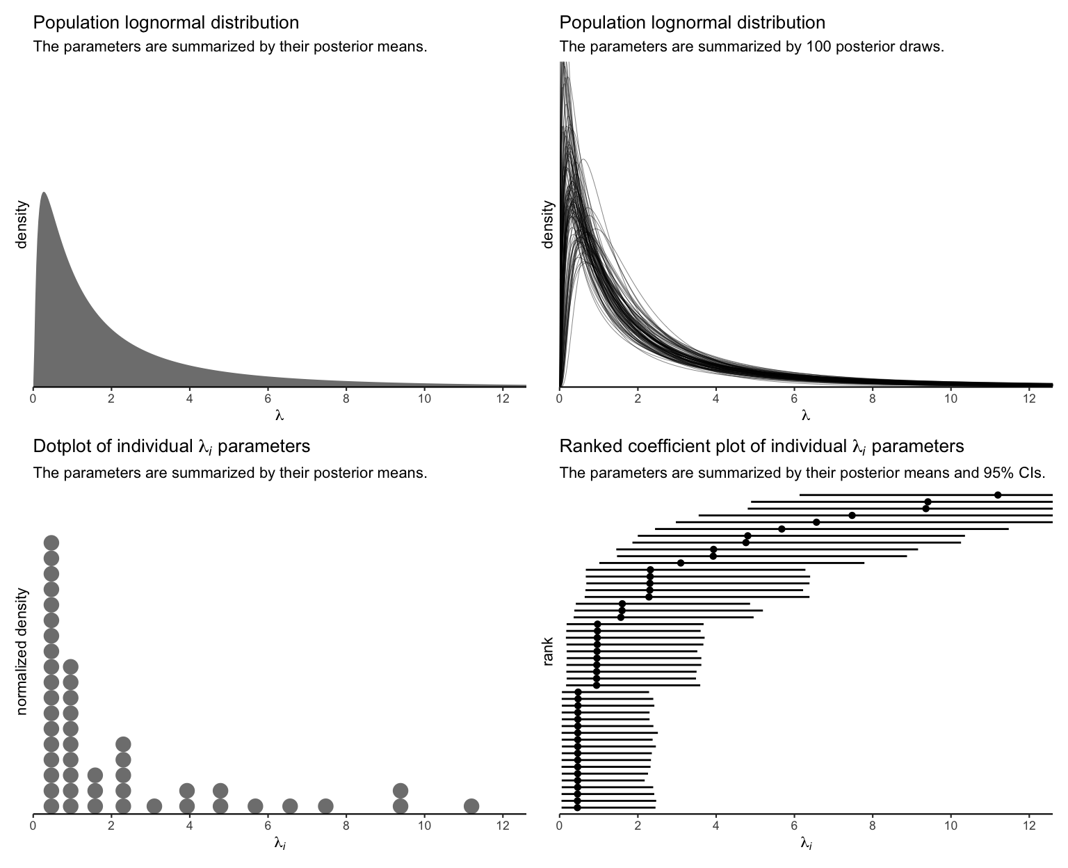
  labs(title = "Population lognormal distribution",
       subtitle = "The parameters are summarized by their posterior means.")

p1

Using just the posterior means for the parameters ignores the uncertainty in the distribution. To bring that into the plot, we’ll want to work with the posterior samples, themselves.

# how many posterior draws would you like?
n_draw <- 100

set.seed(1)

p2 <-
  as_draws_df(fit3) %>% 
  slice_sample(n = n_draw) %>% 
  transmute(iter  = 1:n(),
            mu    = b_Intercept,
            sigma = sd_SITE__Intercept) %>% 
  expand(nesting(iter, mu, sigma),
         lambda = seq(from = 0, to = 13, length.out = 500)) %>% 
  mutate(d = dlnorm(lambda, meanlog = mu, sdlog = sigma)) %>% 
  
  ggplot(aes(x = lambda, y = d, group = iter)) +
  geom_line(linewidth = 1/6, alpha = 1/2) +
  scale_x_continuous(expression(lambda), breaks = 0:6 * 2, 
                     expand = expansion(mult = c(0, 0.05))) +
  scale_y_continuous("density", breaks = NULL, 
                     expand = expansion(mult = c(0, 0.05))) +
  coord_cartesian(xlim = c(0, 12),
                  ylim = c(0, 0.8)) +
  labs(title = "Population lognormal distribution",
       subtitle = "The parameters are summarized by 100 posterior draws.")

p2

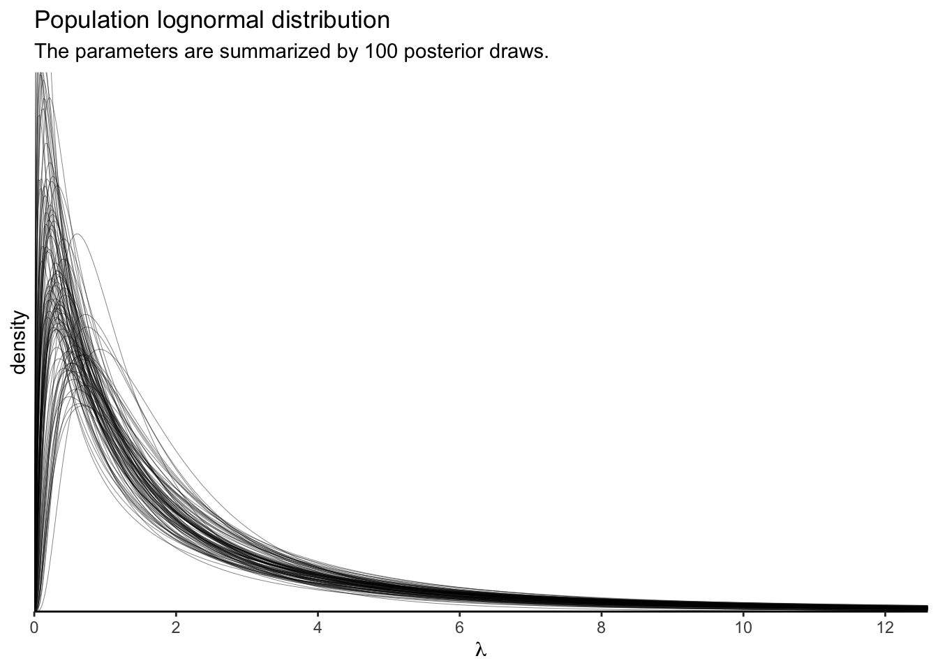
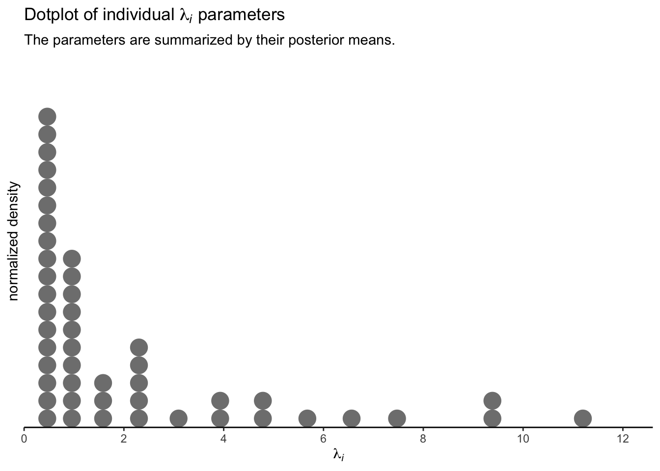
These, recall, are 100 credible lognormal distributions for the case-level \(\lambda_i\) parameters, not for the data themselves. We’ll get to the data in a moment. Since we’re working with a multilevel model, we have posteriors for each of the case-level \(\lambda_i\) parameters, too. Here they are in a dot plot.

p3 <-
  coef(fit3)$SITE[, "Estimate", "Intercept"] %>% 
  exp() %>% 
  data.frame() %>% 
  set_names("lambda_i") %>% 
  
  ggplot(aes(x = lambda_i)) +
  geom_dots(fill = "grey50", color = "grey50") +
  scale_x_continuous(expression(lambda[italic(i)]), breaks = 0:6 * 2, 
                     expand = expansion(mult = c(0, 0.05))) +
  scale_y_continuous("normalized density", breaks = NULL, 
                     expand = expansion(mult = c(0, 0.05))) +
  coord_cartesian(xlim = c(0, 12)) +
  labs(title = expression("Dotplot of individual "*lambda[italic(i)]*" parameters"),
       subtitle = "The parameters are summarized by their posterior means.")

p3

To reduce visual complexity, we just plotted the \(\lambda_i\) parameters by their posterior means. But that might be frustrating the way it ignores uncertainty. A different way to look at them might be a rank-ordered coefficient plot.

p4 <-
  coef(fit3)$SITE[, -2, "Intercept"] %>% 
  exp() %>% 
  data.frame() %>% 
  arrange(Estimate) %>% 
  mutate(rank = 1:n()) %>% 
  
  ggplot(aes(x = Estimate, xmin = Q2.5, xmax = Q97.5, y = rank)) +
  geom_pointrange(fatten = 1, linewidth = 1/2) +
  scale_x_continuous(expression(lambda[italic(i)]), breaks = 0:6 * 2, 
                     expand = expansion(mult = c(0, 0.05))) +
  scale_y_continuous(breaks = NULL, expand = c(0.02, 0.02)) +
  coord_cartesian(xlim = c(0, 12)) +
  labs(title = expression("Ranked coefficient plot of individual "*lambda[italic(i)]*" parameters"),
       subtitle = "The parameters are summarized by their posterior means and 95% CIs.")

p4

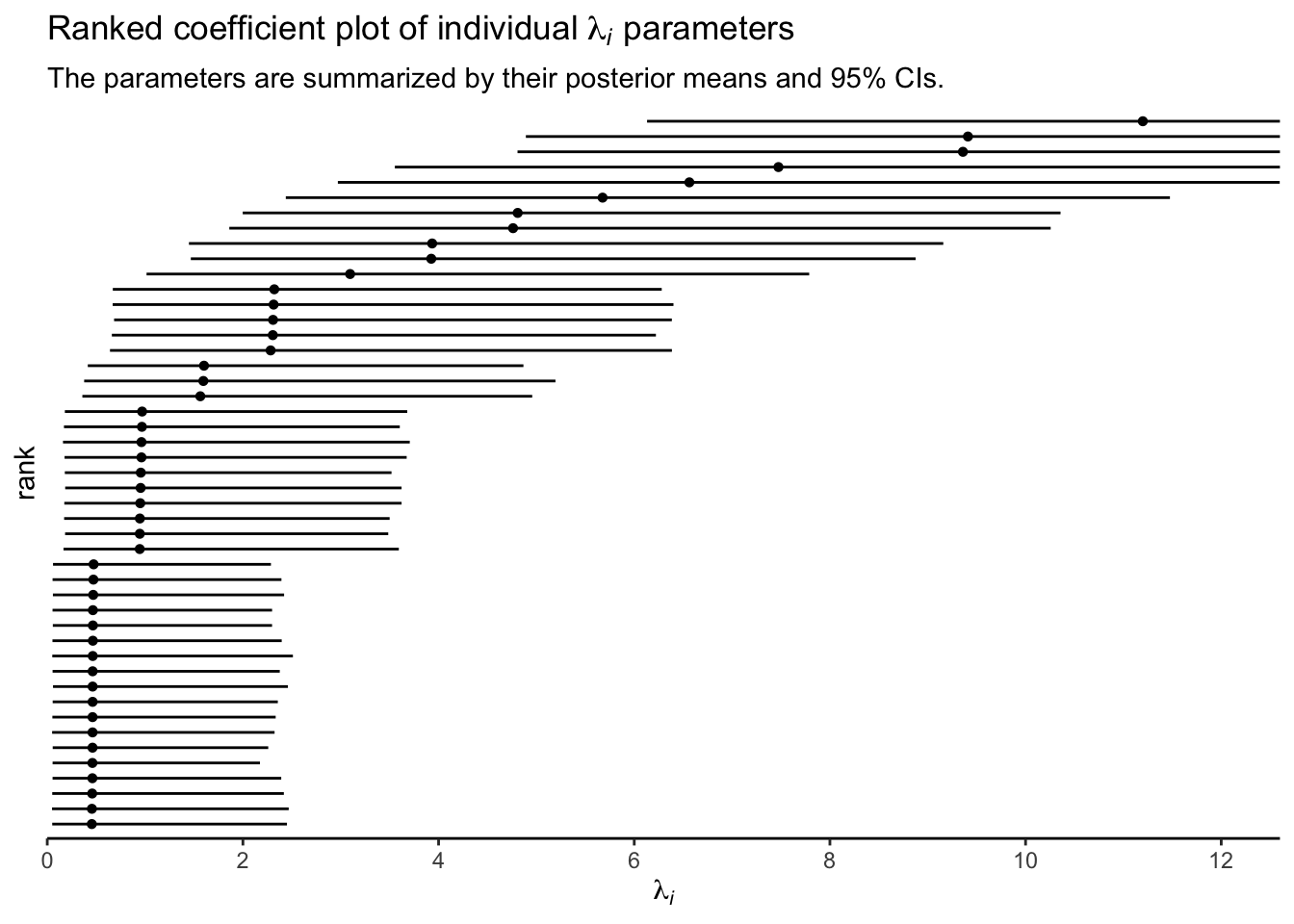
Since each \(\lambda_i\) parameter is based in the data from a single case, it’s no surprise that their 95% intervals are all on the wide side. Just for kicks, here are the last four subplots all shown together.

p1 + p2 + p3 + p4 & 
  theme_classic(base_size = 8.25)

At this point, though, you may be wondering how this model, with all its lognormal \(\lambda_i\) glory, can inform us about actual counts. You know, the kind of counts that allowed us to fit such a wacky model. We’ll want to work with the posterior draws for that, too. First we extract all of the posterior draws for the population parameters.

draws <-
  as_draws_df(fit3) %>% 
  transmute(mu    = b_Intercept,
            sigma = sd_SITE__Intercept)

# what is this?
glimpse(draws)

## Rows: 4,000
## Columns: 2
## $ mu    <dbl> 0.16424013, 0.07509823, 0.26418683, 0.22422613, 0.36427113, -0.1…
## $ sigma <dbl> 1.4128424, 1.4236003, 1.2986505, 1.4523181, 1.2731463, 1.5761309…

The next code block is a little chunky, so I’ll try to explain what we’re doing before we dive in. Our goal is to use the posterior draws to make a posterior predictive check, by hand. My reasoning is doing this kind of check by hand, rather than relying on pp_check(), requires you to understand the guts of the model. In our check, we are going to compare the histogram of the original SALAMAN counts with the histograms of a few data sets simulated from the model. So first, we need to decide how many simulations we want. Since I want a faceted plot of 12 histograms, that means we’ll need 11 simulations. We set that number with the opening n_facet <- 12 line. Next, we set our seed for reproducibility and took 11 random draws from the post data frame. In the first mutate() line, we added an iteration index. Then with the purrr::map2() function, we drew 47 \(\lambda\) values (47 was the original \(N\) in the salamanders data) based on the lognormal distribution defined by the \(\mu\) and \(\sigma\) values from each iteration. After unnest()-ing those results, we used rpois() within the next mutate() line to use those simulated \(\lambda\) values to simulate actual counts. The remaining lines clean up the data format a bit and tack on the original salamanders data. Then we plot.

Okay, here it is:

# how many facets would you like?
n_facet <- 12

set.seed(1)

draws %>% 
  # take 11 samples from the posterior iterations
  slice_sample(n = n_facet - 1) %>% 
  # take 47 random draws from each iteration
  mutate(iter   = 1:n(),
         lambda = map2(mu, sigma, ~ rlnorm(n = 47, meanlog = mu, sdlog = sigma))) %>% 
  unnest(lambda) %>% 
  # use the lambdas to generate the counts
  mutate(count = rpois(n(), lambda = lambda)) %>% 
  transmute(sample = str_c("sample #", iter),
            SALAMAN = count) %>% 
  # combine the original data
  bind_rows(
    salamanders %>% 
      select(SALAMAN) %>% 
      mutate(sample = "original data")
  ) %>% 
  
  # plot!
  ggplot(aes(x = SALAMAN, fill = sample == "original data")) +
  geom_bar() +
  scale_fill_viridis_d(option = "A", begin = .15, end = .55, breaks = NULL) +
  scale_y_continuous(NULL, breaks = NULL) +
  coord_cartesian(xlim = c(0, 30)) +
  labs(title = "Handmade posterior predictive check") +
  facet_wrap(~sample) +
  theme(strip.background = element_rect(linewidth = 0, fill = "grey92"))

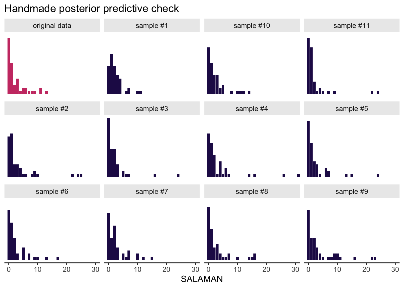
This, friends, is how you can use our intercepts-only Poisson-lognormal mixture model to simulate count data resembling the original count data. Data simulation is cool, but you might wonder how to compute the mean of the model-implied lognormal distribution. Recall that we can’t just exponentiate the model’s intercept. As it turns out, \(\exp \mu\) returns the median for the lognormal distribution. The formula for the mean of the lognormal distribution is

$$\text{mean} = \exp \left ( \mu + \frac{\sigma^2}{2}\right).$$

So here’s how to work with the posterior draws to compute that value.

draws %>% 
  mutate(mean = exp(mu + sigma^2 / 2)) %>% 
  
  ggplot(aes(x = mean, y = 0)) +
  stat_halfeye(.width = c(.5, .95)) +
  geom_vline(xintercept = mean(salamanders$SALAMAN), 
             color = "purple4", linetype = 2) +
  scale_y_continuous(NULL, breaks = NULL) +
  coord_cartesian(xlim = c(0, 10)) +
  xlab(expression("mean of the lognormal "*lambda*" distribution"))

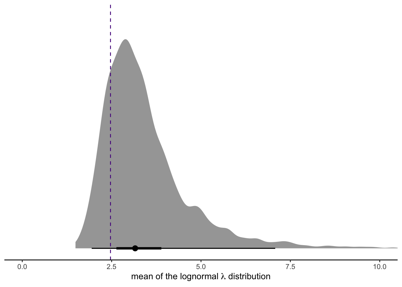
For reference, we superimposed the mean of the SALAMAN data with a dashed line.

Wrap-up

Okay, this is about as far as I’d like to go with this one. To be honest, the Poisson-lognormal mixture is a weird model and I’m not sure if it’s a good fit for the kind of data I tend to work with. But exposure to new options seems valuable and I’m content to low-key chew on this one for a while.

If you’d like to learn more, do check out Bulmer’s original ( 1974) paper and the more recent OLRE paper by Harrison ( 2014). The great Ben Bolker wrote up a vignette ( here) on how to fit the OLRE Poisson-lognormal with lme4 ( Bates et al., 2021) and Michael Clark wrote up a very quick example of the model with brms here.

Happy modeling.

Session info

sessionInfo()

## R version 4.2.0 (2022-04-22)
## Platform: x86_64-apple-darwin17.0 (64-bit)
## Running under: macOS Big Sur/Monterey 10.16
## 
## Matrix products: default
## BLAS:   /Library/Frameworks/R.framework/Versions/4.2/Resources/lib/libRblas.0.dylib
## LAPACK: /Library/Frameworks/R.framework/Versions/4.2/Resources/lib/libRlapack.dylib
## 
## locale:
## [1] en_US.UTF-8/en_US.UTF-8/en_US.UTF-8/C/en_US.UTF-8/en_US.UTF-8
## 
## attached base packages:
## [1] stats     graphics  grDevices utils     datasets  methods   base     
## 
## other attached packages:
##  [1] patchwork_1.1.2 tidybayes_3.0.2 forcats_0.5.1   stringr_1.4.1  
##  [5] dplyr_1.0.10    purrr_0.3.4     readr_2.1.2     tidyr_1.2.1    
##  [9] tibble_3.1.8    ggplot2_3.4.0   tidyverse_1.3.2 brms_2.18.0    
## [13] Rcpp_1.0.9     
## 
## loaded via a namespace (and not attached):
##   [1] readxl_1.4.1         backports_1.4.1      plyr_1.8.7          
##   [4] igraph_1.3.4         svUnit_1.0.6         splines_4.2.0       
##   [7] crosstalk_1.2.0      TH.data_1.1-1        rstantools_2.2.0    
##  [10] inline_0.3.19        digest_0.6.30        htmltools_0.5.3     
##  [13] fansi_1.0.3          magrittr_2.0.3       checkmate_2.1.0     
##  [16] googlesheets4_1.0.1  tzdb_0.3.0           modelr_0.1.8        
##  [19] RcppParallel_5.1.5   matrixStats_0.62.0   xts_0.12.1          
##  [22] sandwich_3.0-2       prettyunits_1.1.1    colorspace_2.0-3    
##  [25] rvest_1.0.2          ggdist_3.2.0         haven_2.5.1         
##  [28] xfun_0.35            callr_3.7.3          crayon_1.5.2        
##  [31] jsonlite_1.8.3       lme4_1.1-31          survival_3.4-0      
##  [34] zoo_1.8-10           glue_1.6.2           gtable_0.3.1        
##  [37] gargle_1.2.0         emmeans_1.8.0        distributional_0.3.1
##  [40] pkgbuild_1.3.1       rstan_2.21.7         abind_1.4-5         
##  [43] scales_1.2.1         mvtnorm_1.1-3        DBI_1.1.3           
##  [46] miniUI_0.1.1.1       viridisLite_0.4.1    xtable_1.8-4        
##  [49] stats4_4.2.0         StanHeaders_2.21.0-7 DT_0.24             
##  [52] htmlwidgets_1.5.4    httr_1.4.4           threejs_0.3.3       
##  [55] arrayhelpers_1.1-0   posterior_1.3.1      ellipsis_0.3.2      
##  [58] pkgconfig_2.0.3      loo_2.5.1            farver_2.1.1        
##  [61] sass_0.4.2           dbplyr_2.2.1         utf8_1.2.2          
##  [64] labeling_0.4.2       tidyselect_1.1.2     rlang_1.0.6         
##  [67] reshape2_1.4.4       later_1.3.0          munsell_0.5.0       
##  [70] cellranger_1.1.0     tools_4.2.0          cachem_1.0.6        
##  [73] cli_3.4.1            generics_0.1.3       broom_1.0.1         
##  [76] ggridges_0.5.3       evaluate_0.18        fastmap_1.1.0       
##  [79] yaml_2.3.5           processx_3.8.0       knitr_1.40          
##  [82] fs_1.5.2             nlme_3.1-159         mime_0.12           
##  [85] projpred_2.2.1       xml2_1.3.3           compiler_4.2.0      
##  [88] bayesplot_1.9.0      shinythemes_1.2.0    rstudioapi_0.13     
##  [91] gamm4_0.2-6          reprex_2.0.2         bslib_0.4.0         
##  [94] stringi_1.7.8        highr_0.9            ps_1.7.2            
##  [97] blogdown_1.15        Brobdingnag_1.2-8    lattice_0.20-45     
## [100] Matrix_1.4-1         nloptr_2.0.3         markdown_1.1        
## [103] shinyjs_2.1.0        tensorA_0.36.2       vctrs_0.5.0         
## [106] pillar_1.8.1         lifecycle_1.0.3      jquerylib_0.1.4     
## [109] bridgesampling_1.1-2 estimability_1.4.1   httpuv_1.6.5        
## [112] R6_2.5.1             bookdown_0.28        promises_1.2.0.1    
## [115] gridExtra_2.3        codetools_0.2-18     boot_1.3-28         
## [118] colourpicker_1.1.1   MASS_7.3-58.1        gtools_3.9.3        
## [121] assertthat_0.2.1     withr_2.5.0          shinystan_2.6.0     
## [124] multcomp_1.4-20      mgcv_1.8-40          parallel_4.2.0      
## [127] hms_1.1.1            grid_4.2.0           coda_0.19-4         
## [130] minqa_1.2.5          rmarkdown_2.16       googledrive_2.0.0   
## [133] shiny_1.7.2          lubridate_1.8.0      base64enc_0.1-3     
## [136] dygraphs_1.1.1.6

References

Bates, D., Maechler, M., Bolker, B., & Steven Walker. (2022). lme4: Linear mixed-effects models using Eigen’ and S4. https://CRAN.R-project.org/package=lme4
Bulmer, M. (1974). On fitting the Poisson lognormal distribution to species-abundance data. Biometrics. Journal of the International Biometric Society, 30(1), 101–110. https://doi.org/10.2307/2529621
Bürkner, P.-C. (2017). brms: An R package for Bayesian multilevel models using Stan. Journal of Statistical Software, 80(1), 1–28. https://doi.org/10.18637/jss.v080.i01
Bürkner, P.-C. (2018). Advanced Bayesian multilevel modeling with the R package brms. The R Journal, 10(1), 395–411. https://doi.org/10.32614/RJ-2018-017
Bürkner, P.-C. (2021a). Estimating distributional models with brms. https://CRAN.R-project.org/package=brms/vignettes/brms_distreg.html
Bürkner, P.-C. (2021b). Parameterization of response distributions in brms. https://CRAN.R-project.org/package=brms/vignettes/brms_families.html
Bürkner, P.-C. (2022). brms: Bayesian regression models using ’Stan’. https://CRAN.R-project.org/package=brms
Cameron, A. C., & Trivedi, P. K. (2013). Regression analysis of count data (Second Edition). Cambridge University Press. https://doi.org/10.1017/CBO9781139013567
Gelman, A., & Hill, J. (2006). Data analysis using regression and multilevel/hierarchical models. Cambridge University Press. https://doi.org/10.1017/CBO9780511790942
Harrison, X. A. (2014). Using observation-level random effects to model overdispersion in count data in ecology and evolution. PeerJ, 2, e616. https://doi.org/10.7717/peerj.616
Hilbe, J. M. (2011). Negative binomial regression (Second Edition). https://doi.org/10.1017/CBO9780511973420
Kay, M. (2023). tidybayes: Tidy data and ’geoms’ for Bayesian models. https://CRAN.R-project.org/package=tidybayes
McElreath, R. (2020a). rethinking R package. https://xcelab.net/rm/software/
McElreath, R. (2020b). Statistical rethinking: A Bayesian course with examples in R and Stan (Second Edition). CRC Press. https://xcelab.net/rm/statistical-rethinking/
Pedersen, T. L. (2022). patchwork: The composer of plots. https://CRAN.R-project.org/package=patchwork
R Core Team. (2022). R: A language and environment for statistical computing. R Foundation for Statistical Computing. https://www.R-project.org/
Stan Development Team. (2021). Stan functions reference. https://mc-stan.org/docs/2_26/functions-reference/index.html
Welsh Jr, H. H., & Lind, A. J. (1995). Habitat correlates of the Del Norte salamander, Plethodon elongatus (Caudata: Plethodontidae), in northwestern California. Journal of Herpetology, 29(2), 198–210. https://doi.org/10.2307/1564557
Wickham, H. (2022). tidyverse: Easily install and load the ’tidyverse’. https://CRAN.R-project.org/package=tidyverse
Wickham, H., Averick, M., Bryan, J., Chang, W., McGowan, L. D., François, R., Grolemund, G., Hayes, A., Henry, L., Hester, J., Kuhn, M., Pedersen, T. L., Miller, E., Bache, S. M., Müller, K., Ooms, J., Robinson, D., Seidel, D. P., Spinu, V., … Yutani, H. (2019). Welcome to the tidyverse. Journal of Open Source Software, 4(43), 1686. https://doi.org/10.21105/joss.01686
-
Older versions of this post included an embedded link showing Mahr’s tweet. Mahr has since made his account private, and the code no longer works to share his tweet. Though this breaks the flow of the blog a little, and it removes some of the charm, I hope you can still follow the main point. Mahr said some smart things on social media, I found it surprising, and that exchange led to this blog post. ↩︎
That’s a lie. There was no pop quiz, last week. ↩︎
I’m making this number up, too, but it’s probably not far off. ☕ ☕ ☕ ↩︎
One could also, of course, express that model as
\(y_i = \beta_0 + \beta_1 x_i + \epsilon_i\), where\(\epsilon_i \sim \operatorname{Normal}(0, \sigma)\). But come on. That’s weak sauce. For more on why, see page 84 in McElreath ( 2020b). ↩︎ -
I say “suggests” because a simple Poisson model can be good enough IF you have a set of high-quality predictors which can “explain” all that extra-looking variability. We, however, will be fitting intercept-only models. ↩︎
- Posted on:
- July 12, 2021
- Length:
- 24 minute read, 5103 words