Sum-score effect sizes for multilevel Bayesian cumulative probit models

What/why?

This is a follow-up to my earlier post, Notes on the Bayesian cumulative probit. If you haven’t browsed through that post or if you aren’t at least familiar with Bayesian cumulative probit models, you’ll want to go there, first. Comparatively speaking, this post will be short and focused. The topic we’re addressing is: After you fit a full multilevel Bayesian cumulative probit model of several Likert-type items from a multi-item questionnaire, how can you use the model to compute an effect size in the sum-score metric?

Needless to say, I’m assuming my readers are familiar with the Bayesian generalized linear mixed model, in general, and with ordinal models in particular. For a refresher on the latter, check out Bürkner & Vuorre ( 2019) and Bürkner ( 2020).

Set it up

All code is in R ( R Core Team, 2022), with healthy doses of the tidyverse ( Wickham et al., 2019; Wickham, 2022) for data wrangling and plotting. All models are fit with brms ( Bürkner, 2017, 2018, 2022) and we’ll make use of the tidybayes package ( Kay, 2022) for some tricky data wrangling. We will also use the NatParksPalettes package ( Blake, 2022) to select the color palette for our figures.

Here we load the packages and adjust the global plotting theme.

# load
library(tidyverse)
library(brms)
library(tidybayes)

# save a color vector
npp <- NatParksPalettes::natparks.pals("Olympic", n = 41)

# adjust the global plotting theme
theme_set(
  theme_grey(base_size = 14,
             base_family = "Times") +
    theme(text = element_text(color = npp[1]),
          axis.text = element_text(color = npp[1]),
          axis.ticks = element_line(color = npp[1]),
          panel.background = element_rect(fill = npp[21], color = npp[21]),
          panel.grid = element_blank(),
          plot.background = element_rect(fill = alpha(npp[21], alpha = .5), 
                                         color = alpha(npp[21], alpha = .5)),
          strip.background = element_rect(fill = npp[23]),
          strip.text = element_text(color = npp[1]))
)

Our data will be a subset of the bfi data ( Revelle et al., 2010) from the psych package ( Revelle, 2022). Here we load, subset, and wrangle the data to suit our needs.

set.seed(1)

d <- psych::bfi %>% 
  mutate(male = ifelse(gender == 1, 1, 0),
         female = ifelse(gender == 2, 1, 0)) %>% 
  drop_na() %>% 
  slice_sample(n = 200) %>% 
  mutate(id = 1:n()) %>% 
  select(id, male, female, N1:N5) %>% 
  pivot_longer(N1:N5, names_to = "item", values_to = "rating")

# what is this?
glimpse(d)

## Rows: 1,000
## Columns: 5
## $ id     <int> 1, 1, 1, 1, 1, 2, 2, 2, 2, 2, 3, 3, 3, 3, 3, 4, 4, 4, 4, 4, 5, 5, 5, 5, 5, 6, 6, 6, 6, 6, 7, 7, 7, 7, 7…
## $ male   <dbl> 1, 1, 1, 1, 1, 1, 1, 1, 1, 1, 0, 0, 0, 0, 0, 1, 1, 1, 1, 1, 0, 0, 0, 0, 0, 0, 0, 0, 0, 0, 0, 0, 0, 0, 0…
## $ female <dbl> 0, 0, 0, 0, 0, 0, 0, 0, 0, 0, 1, 1, 1, 1, 1, 0, 0, 0, 0, 0, 1, 1, 1, 1, 1, 1, 1, 1, 1, 1, 1, 1, 1, 1, 1…
## $ item   <chr> "N1", "N2", "N3", "N4", "N5", "N1", "N2", "N3", "N4", "N5", "N1", "N2", "N3", "N4", "N5", "N1", "N2", "…
## $ rating <int> 2, 2, 1, 1, 1, 3, 3, 2, 3, 3, 4, 4, 4, 4, 2, 5, 3, 4, 6, 2, 1, 1, 3, 2, 2, 2, 4, 4, 1, 2, 1, 2, 4, 4, 1…

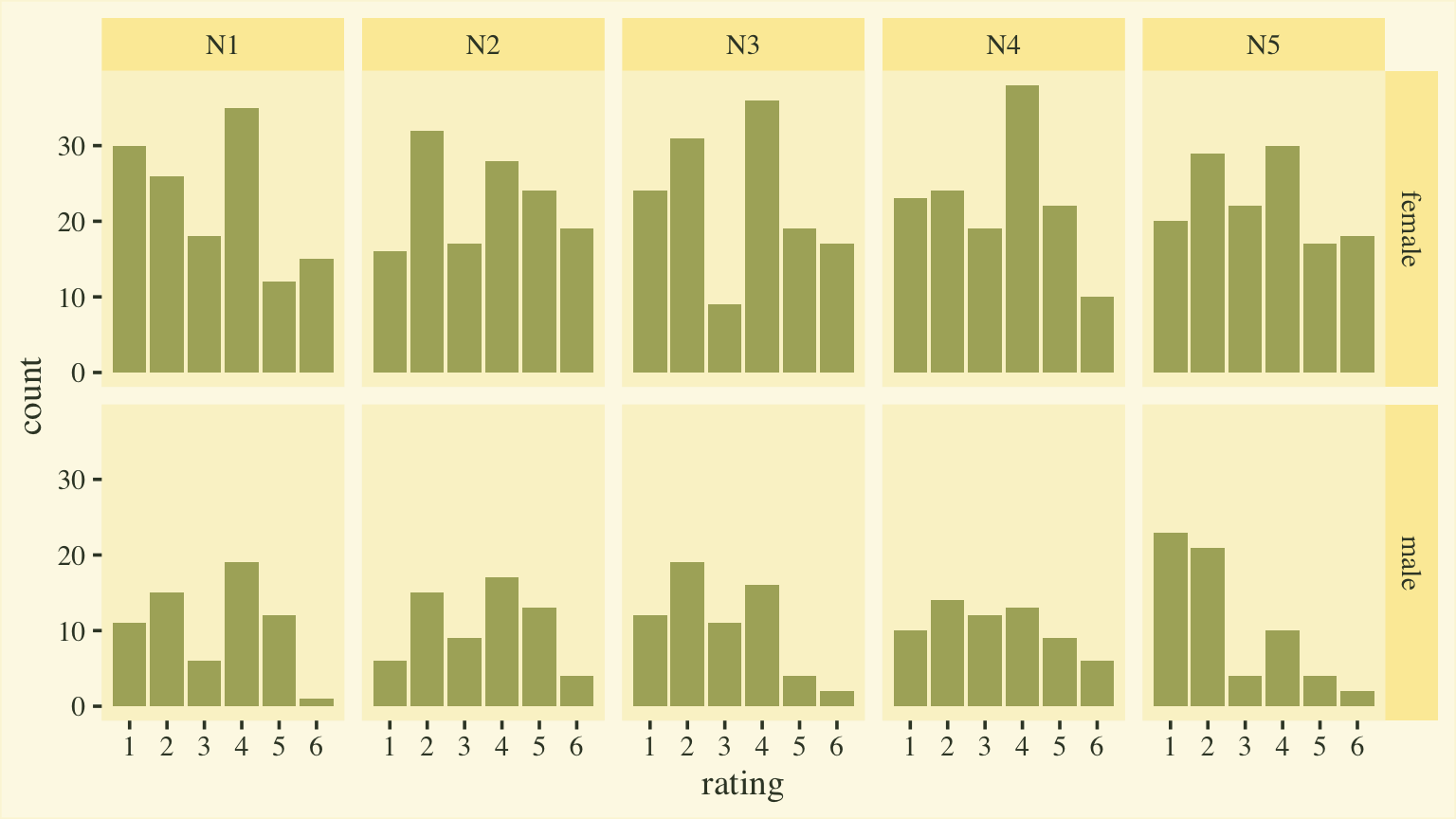
Our focal variables will be rating, which is a combination of the responses to the five questions in the Neuroticism scale of a version of the Big Five inventory ( Goldberg, 1999). Here’s a quick plot of the responses, by item and sex.

d %>% 
  mutate(sex = ifelse(male == 0, "female", "male")) %>% 
  
  ggplot(aes(x = rating)) +
  geom_bar(fill = npp[15]) +  
  scale_x_continuous(breaks = 1:6) +
  facet_grid(sex ~ item)

Model

In the earlier post, we explored eight different cumulative probit models for the neuroticism data. Here, we’ll jump straight to the final model, fit8, which we described as a multilevel conditional distributional model. When the data are in the long format, we can describe the criterion variable rating, as varying across \(i\) persons, \(j\) items, and \(k\) Likert-type rating options, with the model

$$ \begin{align*} \small{p(\text{rating} = k | \{ \tau_{kj} \}, \mu_{ij}, \alpha_{ij})} & = \small{\Phi(\alpha_{ij}[\tau_{kj} - \mu_{ij}]) - \Phi(\alpha_{ij}[\tau_{k - 1,j} - \mu_{ij}])} \\ \mu_{ij} & = \beta_1 \text{male}_i + u_i + v_j \\ \log(\alpha_{ij}) & = \eta_1 \text{male}_i + w_i + x_j \\ u_i & \sim \mathcal N(0, \sigma_u) \\ v_j & \sim \mathcal N(0, \sigma_v) \\ w_i & \sim \mathcal N(0, \sigma_w) \\ x_j & \sim \mathcal N(0, \sigma_x) \\ \tau_{1j} & \sim \mathcal N(-0.97, 1) \\ \tau_{2j} & \sim \mathcal N(-0.43, 1) \\ \tau_{3j} & \sim \mathcal N(0, 1) \\ \tau_{4j} & \sim \mathcal N(0.43, 1) \\ \tau_{5j} & \sim \mathcal N(0.97, 1) \\ \beta_1 & \sim \mathcal N(0, 1) \\ \eta_1 & \sim \mathcal N(0, 0.347) \\ \sigma_u, \sigma_v & \sim \operatorname{Exponential}(1) \\ \sigma_w, \sigma_x & \sim \operatorname{Exponential}(1 / 0.463), \end{align*} $$

where the only predictor is the dummy variable male. We call this a distributional model because we have attached linear models to both \(\mu_{ij}\) AND \(\log(\alpha_{ij})\). Here’s how to fit the model with brm().

# 2.786367 mins
fit8 <- brm(
  data = d,
  family = cumulative(probit),
  bf(rating | thres(gr = item) ~ 1 + male + (1 | id) + (1 | item)) +
    lf(disc                    ~ 0 + male + (1 | id) + (1 | item),
       # don't forget this line
       cmc = FALSE),
  prior = c(prior(normal(-0.97, 1), class = Intercept, coef = 1, group = N1),
            prior(normal(-0.43, 1), class = Intercept, coef = 2, group = N1),
            prior(normal( 0.00, 1), class = Intercept, coef = 3, group = N1),
            prior(normal( 0.43, 1), class = Intercept, coef = 4, group = N1),
            prior(normal( 0.97, 1), class = Intercept, coef = 5, group = N1),
            
            prior(normal(-0.97, 1), class = Intercept, coef = 1, group = N2),
            prior(normal(-0.43, 1), class = Intercept, coef = 2, group = N2),
            prior(normal( 0.00, 1), class = Intercept, coef = 3, group = N2),
            prior(normal( 0.43, 1), class = Intercept, coef = 4, group = N2),
            prior(normal( 0.97, 1), class = Intercept, coef = 5, group = N2),
            
            prior(normal(-0.97, 1), class = Intercept, coef = 1, group = N3),
            prior(normal(-0.43, 1), class = Intercept, coef = 2, group = N3),
            prior(normal( 0.00, 1), class = Intercept, coef = 3, group = N3),
            prior(normal( 0.43, 1), class = Intercept, coef = 4, group = N3),
            prior(normal( 0.97, 1), class = Intercept, coef = 5, group = N3),
            
            prior(normal(-0.97, 1), class = Intercept, coef = 1, group = N4),
            prior(normal(-0.43, 1), class = Intercept, coef = 2, group = N4),
            prior(normal( 0.00, 1), class = Intercept, coef = 3, group = N4),
            prior(normal( 0.43, 1), class = Intercept, coef = 4, group = N4),
            prior(normal( 0.97, 1), class = Intercept, coef = 5, group = N4),
            
            prior(normal(-0.97, 1), class = Intercept, coef = 1, group = N5),
            prior(normal(-0.43, 1), class = Intercept, coef = 2, group = N5),
            prior(normal( 0.00, 1), class = Intercept, coef = 3, group = N5),
            prior(normal( 0.43, 1), class = Intercept, coef = 4, group = N5),
            prior(normal( 0.97, 1), class = Intercept, coef = 5, group = N5),
            
            prior(normal(0, 1), class = b),
            prior(normal(0, log(2) / 2), class = b, dpar = disc),
            
            prior(exponential(1), class = sd),
            prior(exponential(1 / 0.463), class = sd, dpar = disc)),
  cores = 4,
  seed = 1,
  init_r = 0.2,
  control = list(adapt_delta = .99)
)

You might check the model summary.

print(fit8)

##  Family: cumulative 
##   Links: mu = probit; disc = log 
## Formula: rating | thres(gr = item) ~ 1 + male + (1 | id) + (1 | item) 
##          disc ~ 0 + male + (1 | id) + (1 | item)
##    Data: d (Number of observations: 1000) 
##   Draws: 4 chains, each with iter = 2000; warmup = 1000; thin = 1;
##          total post-warmup draws = 4000
## 
## Group-Level Effects: 
## ~id (Number of levels: 200) 
##                    Estimate Est.Error l-95% CI u-95% CI Rhat Bulk_ESS Tail_ESS
## sd(Intercept)          1.21      0.14     0.94     1.50 1.00      590      972
## sd(disc_Intercept)     0.45      0.06     0.34     0.56 1.00     1264     2045
## 
## ~item (Number of levels: 5) 
##                    Estimate Est.Error l-95% CI u-95% CI Rhat Bulk_ESS Tail_ESS
## sd(Intercept)          0.23      0.21     0.01     0.77 1.00     1642     2421
## sd(disc_Intercept)     0.39      0.19     0.14     0.84 1.00      899     1094
## 
## Population-Level Effects: 
##                 Estimate Est.Error l-95% CI u-95% CI Rhat Bulk_ESS Tail_ESS
## Intercept[N1,1]    -1.42      0.30    -2.06    -0.87 1.00      852     1998
## Intercept[N1,2]    -0.58      0.25    -1.13    -0.10 1.00     1371     2291
## Intercept[N1,3]    -0.13      0.24    -0.66     0.32 1.00     2017     2668
## Intercept[N1,4]     1.00      0.27     0.42     1.52 1.00     2255     2633
## Intercept[N1,5]     1.91      0.33     1.25     2.56 1.00     1656     2425
## Intercept[N2,1]    -1.93      0.34    -2.59    -1.28 1.00      883     1688
## Intercept[N2,2]    -0.69      0.26    -1.17    -0.12 1.00     1439     2290
## Intercept[N2,3]    -0.20      0.24    -0.67     0.36 1.00     1901     2594
## Intercept[N2,4]     0.63      0.25     0.16     1.19 1.00     2065     2259
## Intercept[N2,5]     1.64      0.31     1.07     2.29 1.00     1384     2180
## Intercept[N3,1]    -1.58      0.32    -2.29    -1.00 1.00      980     1920
## Intercept[N3,2]    -0.42      0.25    -0.98     0.04 1.00     1915     2612
## Intercept[N3,3]    -0.02      0.25    -0.58     0.42 1.00     2570     2990
## Intercept[N3,4]     1.13      0.28     0.55     1.66 1.00     2270     2796
## Intercept[N3,5]     2.05      0.36     1.34     2.78 1.00     1693     2408
## Intercept[N4,1]    -1.96      0.37    -2.74    -1.30 1.00      815     1477
## Intercept[N4,2]    -0.80      0.28    -1.40    -0.28 1.00     1473     2165
## Intercept[N4,3]    -0.09      0.26    -0.61     0.41 1.00     2474     3005
## Intercept[N4,4]     1.15      0.30     0.54     1.74 1.00     2335     2819
## Intercept[N4,5]     2.51      0.43     1.71     3.39 1.00     1422     2364
## Intercept[N5,1]    -1.69      0.35    -2.43    -1.07 1.00     1006     1560
## Intercept[N5,2]    -0.39      0.27    -1.00     0.07 1.00     2144     2503
## Intercept[N5,3]     0.20      0.26    -0.40     0.68 1.00     2847     2723
## Intercept[N5,4]     1.34      0.31     0.70     1.95 1.00     2270     2831
## Intercept[N5,5]     2.33      0.41     1.56     3.19 1.00     1533     2676
## male               -0.31      0.19    -0.70     0.07 1.01      516     1044
## disc_male           0.07      0.10    -0.13     0.27 1.00     1871     2728
## 
## Draws were sampled using sampling(NUTS). For each parameter, Bulk_ESS
## and Tail_ESS are effective sample size measures, and Rhat is the potential
## scale reduction factor on split chains (at convergence, Rhat = 1).

Before we get into the sum-score effect sizes, we might point out that the fit8 model summary provides two effect sizes on the latent Gaussian scale. The reference category, female, follows a normal distribution with a mean of zero and standard deviation of 1. When you use the cumulative probit, these constraints identify an otherwise unidentified model. The \(\beta_1\) parameter is the latent mean difference in neuroticism for males, relative to females. If this was not a full distributional model containing a submodel for \(\log(\alpha_{ij})\), we could interpret \(\beta_1\) like a latent Cohen’s \(d\) standardized mean difference. But we do have a submodel for \(\log(\alpha_{ij})\), which complicates the interpretation a bit. To clarify, first we’ll transform the posteriors for \(\log(\alpha_{ij})\) for the two levels of the male dummy into the latent \(\sigma\) scale. Here’s what they look like.

# extract the posterior draws
post <- as_draws_df(fit8)

# wrangle
post %>% 
  mutate(`sigma[female]` = 1 / exp(0),
         `sigma[male]`   = 1 / exp(b_disc_male)) %>% 
  select(.draw, contains("sigma")) %>% 
  pivot_longer(-.draw) %>% 
  
  # plot
  ggplot(aes(x = value, y = name)) +
  stat_halfeye(.width = .95, fill = npp[14], color = npp[1]) +
  scale_y_discrete(labels = ggplot2:::parse_safe) +
  labs(x = "latent standard deviation (grand means across persons and items)",
       y = NULL)

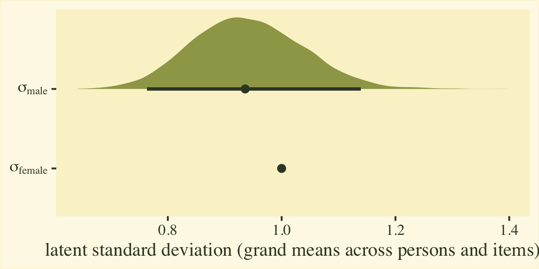
Since \(\eta_0\) was fixed to 0 for identification purposes, the posterior for \(\sigma_\text{female}\) is a constant at 1. We might express that effect size for the latent standard deviations as a difference in \(\sigma\) or a ratio.

post %>% 
  mutate(`sigma[female]` = 1 / exp(0),
         `sigma[male]`   = 1 / exp(b_disc_male)) %>% 
  select(.draw, contains("sigma")) %>% 
  mutate(`sigma[male]-sigma[female]`     = `sigma[male]` - `sigma[female]`,
         `sigma[male]*'/'*sigma[female]` = `sigma[male]` / `sigma[female]`) %>% 
  pivot_longer(`sigma[male]-sigma[female]`:`sigma[male]*'/'*sigma[female]`) %>% 
  
  # plot
  ggplot(aes(x = value, y = name)) +
  geom_vline(xintercept = 0:1, color = npp[26]) +
  stat_halfeye(.width = .95, fill = npp[14], color = npp[1]) +
  scale_y_discrete(labels = ggplot2:::parse_safe) +
  labs(x = "latent standard deviation effect sizes (two ways!)",
       y = NULL)

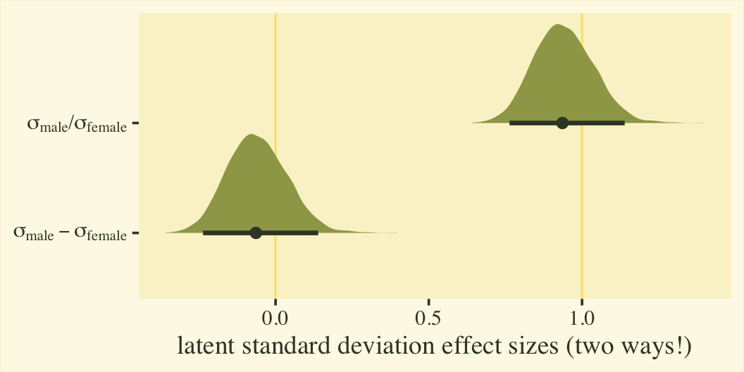
Whether you express the difference as a difference or a ratio, it’s not particularly large. Anyway, now we’re practiced with wrangling those posteriors, we might use them to make a latent pooled standard deviation, with with we might convert our \(\beta_1\) into a proper Cohen’s \(d\).

post %>%
  mutate(`sigma[female]` = 1 / exp(0),
         `sigma[male]`   = 1 / exp(b_disc_male)) %>% 
  # compute the latent pooled standard deviation
  mutate(`sigma[pooled]` = sqrt((`sigma[female]`^2 + `sigma[male]`^2) / 2)) %>% 
  mutate(d = b_male / `sigma[pooled]`) %>% 
    
  ggplot(aes(x = d)) +
  stat_halfeye(.width = .95, fill = npp[14], color = npp[1]) +
  scale_y_continuous(NULL, breaks = NULL) +
  xlab(expression(beta[1]*" converted to a latent Cohen's "*italic(d)))

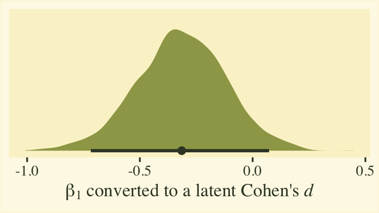
This all has been fun, but we should discuss a few caveats. First, the \(\beta_1\) and \(\eta_1\) have to do with the latent grand means across persons and items. These have relations to sum scores, but they aren’t really sum scores and these kinds of effect sizes aren’t what we’re looking for in this post. Second, latent mean differences like with \(\beta_1\) map on to Cohen’s \(d\) effect sizes reasonably well when you are not using a full distributional model. That is, they work well when you don’t have a submodel for \(\log(\alpha_{ij})\). But once you start fiddling with \(\log(\alpha_{ij})\), the scales of the parameters become difficult to interpret. This is because \(\log(\alpha_{ij})\) doesn’t map directly onto the standard deviations of the criterion variable rating. They’re related, but in a complicated way that’s probably not the most intuitive for non-statisticians or experts in IRT. So this whole latent pooled standard deviation talk is fraught. For more on this, look through some of the plots we made from fit8 in the original blog post.

Okay, let’s get into our sum-score effect sizes.

Sum-score effect sizes

In this post, we will discuss three approaches for reporting sum-score contrasts as effect sizes. Those will include:

• unstandardized mean differences,
• standardized mean differences, and
• differences in POMP.

But before we get to all that effect-size goodness, we’ll first define how we can use our model to compute conditional sum scores, and connect that approach to conditional item-level means.

Condtional sum scores and item-level means.

In the earlier post, we said the mean of the criterion variable is the sum of the \(p_k\) probabilities multiplied by the \(k\) values of the criterion. We can express this in an equation as

$$ \mathbb{E}(\text{rating}) = \sum_1^K p_k \times k, $$

where \(\mathbb{E}\) is the expectation operator (the model-based mean), \(p_k\) is the probability of the \(k^\text{th}\) ordinal value, and \(k\) is the actual ordinal value. Since we have modeled the ordinal rating values of \(j\) items in a multilevel model, we might want to generalize that equation to

$$\mathbb{E}(\text{rating}_j) = \sum_1^K p_{jk} \times k,$$

where the probabilities now vary across \(j\) items and \(k\) rating options. Because we are computing all the \(p_k\) values with MCMC and expressing those values as posterior distributions, we have to perform this operation within each of our MCMC draws. In the earlier post, we practiced this by working directly with the posterior draws returned from brms::as_draws_df(). In this post, we’ll take a short cut with help from the tidybayes::add_epred_draws() function. Here’s a start.

d %>% 
  distinct(item, male) %>% 
  add_epred_draws(fit8, re_formula = ~ (1 | item)) %>% 
  head(n = 10)

## # A tibble: 10 × 8
## # Groups:   male, item, .row, .category [1]
##     male item   .row .chain .iteration .draw .category .epred
##    <dbl> <chr> <int>  <int>      <int> <int> <fct>      <dbl>
##  1     1 N1        1     NA         NA     1 1         0.0502
##  2     1 N1        1     NA         NA     2 1         0.0626
##  3     1 N1        1     NA         NA     3 1         0.0767
##  4     1 N1        1     NA         NA     4 1         0.0650
##  5     1 N1        1     NA         NA     5 1         0.0666
##  6     1 N1        1     NA         NA     6 1         0.0539
##  7     1 N1        1     NA         NA     7 1         0.0661
##  8     1 N1        1     NA         NA     8 1         0.139 
##  9     1 N1        1     NA         NA     9 1         0.0430
## 10     1 N1        1     NA         NA    10 1         0.0654

In that code block, we used the distinct() function to compute the unique combinations of the two variables item and male in the d data. We then used add_epred_draws() to compute the full 4,000-draw posterior distributions for \(p_k\) from each of the five neuroticism items. Note that to compute this by averaging across the levels for participants, we adjusted the settings of the re_formula argument. The draws from \(p_k\) are listed in the .epred column and the levels of \(k\) are listed as a factor in the .category column.

Here’s how to expand on that code to compute \(p_{jk} \times k\) for each posterior draw; sum those products up within each level of item, male, and .draw; convert the results into a sum-scale metric; and then summarize those posteriors by their means and 95% intervals.

posterior_item_means <- d %>% 
  distinct(item, male) %>% 
  add_epred_draws(fit8, re_formula = ~ (1 | item)) %>% 
  # compute p[jk] * k
  mutate(product = as.double(.category) * .epred) %>% 
  # group and convert to the sum-score metric
  group_by(item, male, .draw) %>% 
  summarise(item_mean = sum(product)) %>% 
  # summarize
  group_by(item, male) %>% 
  mean_qi(item_mean)
  
# what?
posterior_item_means

## # A tibble: 10 × 8
##    item   male item_mean .lower .upper .width .point .interval
##    <chr> <dbl>     <dbl>  <dbl>  <dbl>  <dbl> <chr>  <chr>    
##  1 N1        0      3.35   3.06   3.64   0.95 mean   qi       
##  2 N1        1      2.96   2.52   3.41   0.95 mean   qi       
##  3 N2        0      3.67   3.36   3.97   0.95 mean   qi       
##  4 N2        1      3.27   2.82   3.72   0.95 mean   qi       
##  5 N3        0      3.19   2.91   3.46   0.95 mean   qi       
##  6 N3        1      2.84   2.45   3.23   0.95 mean   qi       
##  7 N4        0      3.35   3.10   3.60   0.95 mean   qi       
##  8 N4        1      3.08   2.74   3.42   0.95 mean   qi       
##  9 N5        0      3.07   2.81   3.34   0.95 mean   qi       
## 10 N5        1      2.78   2.41   3.12   0.95 mean   qi

Here we might look at how those posterior summaries compare to the sample means and the sample data in a plot.

# compute and save the sample means
sample_item_means <- d %>% 
  group_by(item, male) %>% 
  summarise(item_mean = mean(rating))

# plot!
d %>%
  ggplot() +
  geom_bar(aes(x = rating),
           fill = npp[15]) +
  geom_pointinterval(data = posterior_item_means,
                     aes(x = item_mean, xmin = .lower, xmax = .upper, y = -1),
                     color = npp[1], size = 1.5) +
  geom_point(data = sample_item_means,
             aes(x = item_mean, y = -3),
             size = 3, shape = 18, color = npp[39]) +
  scale_x_continuous(breaks = 1:6) +
  labs(subtitle = "The mean and 95% intervals for the posterior of each mean are depicted by the dark dots\nand intersecting horizontal lines. The brown diamonds below mark the sample means.",
       y = "count") +
  facet_grid(male ~ item, labeller = label_both)

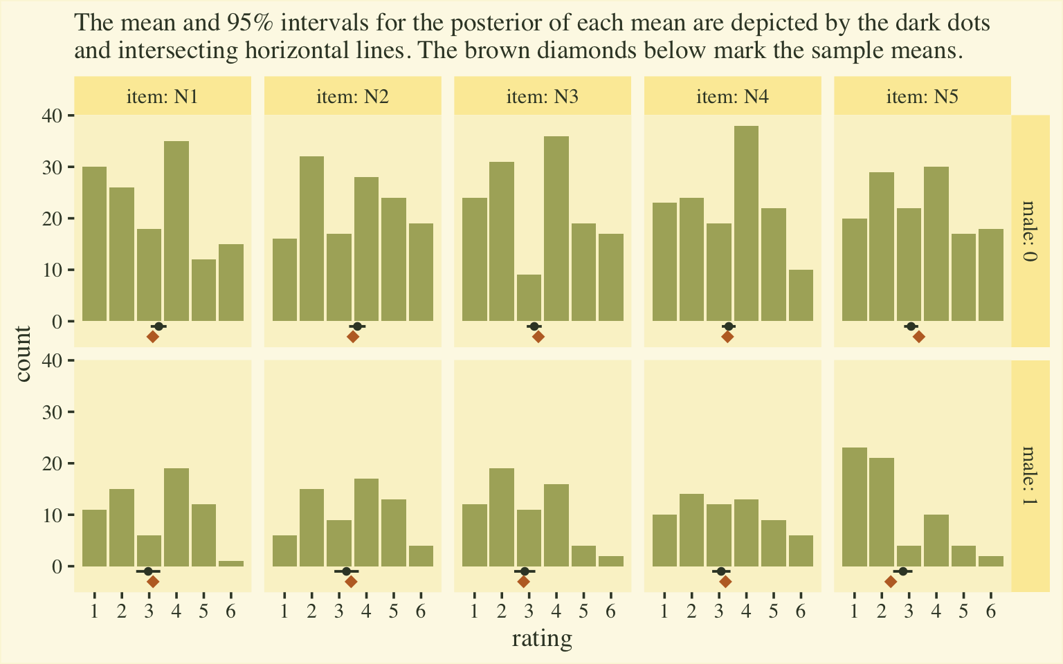
If you’re shaken by the differences in the posterior means and the sample means, keep in mind that the posteriors are based on a multilevel model, which imposed partial pooling across persons and items. The job of the model is to compute the population parameters, not reproduce the sample estimates. To brush up on why we like partial pooling, check out the classic ( 1977) paper by Efron and Morris, Stein’s paradox in statistics, or my blog post on the topic, Stein’s Paradox and what partial pooling can do for you.

Anyway, we only have to make one minor adjustment to our workflow to convert these results into a sum-score metric. In the first group_by() line, we just omit item.

posterior_sum_score_means <- d %>% 
  distinct(item, male) %>% 
  add_epred_draws(fit8, re_formula = ~ (1 | item)) %>% 
  mutate(product = as.double(.category) * .epred) %>% 
  # this line has been changed
  group_by(male, .draw) %>% 
  summarise(sum_score_mean = sum(product)) %>% 
  group_by(male) %>% 
  mean_qi(sum_score_mean)
  
# what?
posterior_sum_score_means

## # A tibble: 2 × 7
##    male sum_score_mean .lower .upper .width .point .interval
##   <dbl>          <dbl>  <dbl>  <dbl>  <dbl> <chr>  <chr>    
## 1     0           16.6   15.5   17.7   0.95 mean   qi       
## 2     1           14.9   13.2   16.7   0.95 mean   qi

As we did with the items, we might look at how those posterior summaries compare to the sample means and the sample data in a plot.

# compute and save the sample means
sample_sum_score_means <- d %>% 
  group_by(id, male, female) %>% 
  summarise(sum_score = sum(rating)) %>% 
  group_by(male) %>% 
  summarise(sum_score_mean = mean(sum_score))

d %>% 
  group_by(id, male, female) %>% 
  summarise(sum_score = sum(rating)) %>% 
  
  ggplot() +
  geom_bar(aes(x = sum_score),
           fill = npp[15]) +
  geom_pointinterval(data = posterior_sum_score_means,
                     aes(x = sum_score_mean, xmin = .lower, xmax = .upper, y = -0.5),
                     color = npp[1], size = 1.75) +
  geom_point(data = sample_sum_score_means,
             aes(x = sum_score_mean, y = -1.2),
             size = 3, shape = 18, color = npp[39]) +
  scale_x_continuous("neuroticism sum score", breaks = c(1, 2, 4, 6) * 5) +
  labs(subtitle = "The mean and 95% intervals for the posterior of each mean are depicted by the dark dots\nand intersecting horizontal lines. The brown diamonds below mark the sample means.",
       y = "count") +
  facet_grid(male ~ ., labeller = label_both)

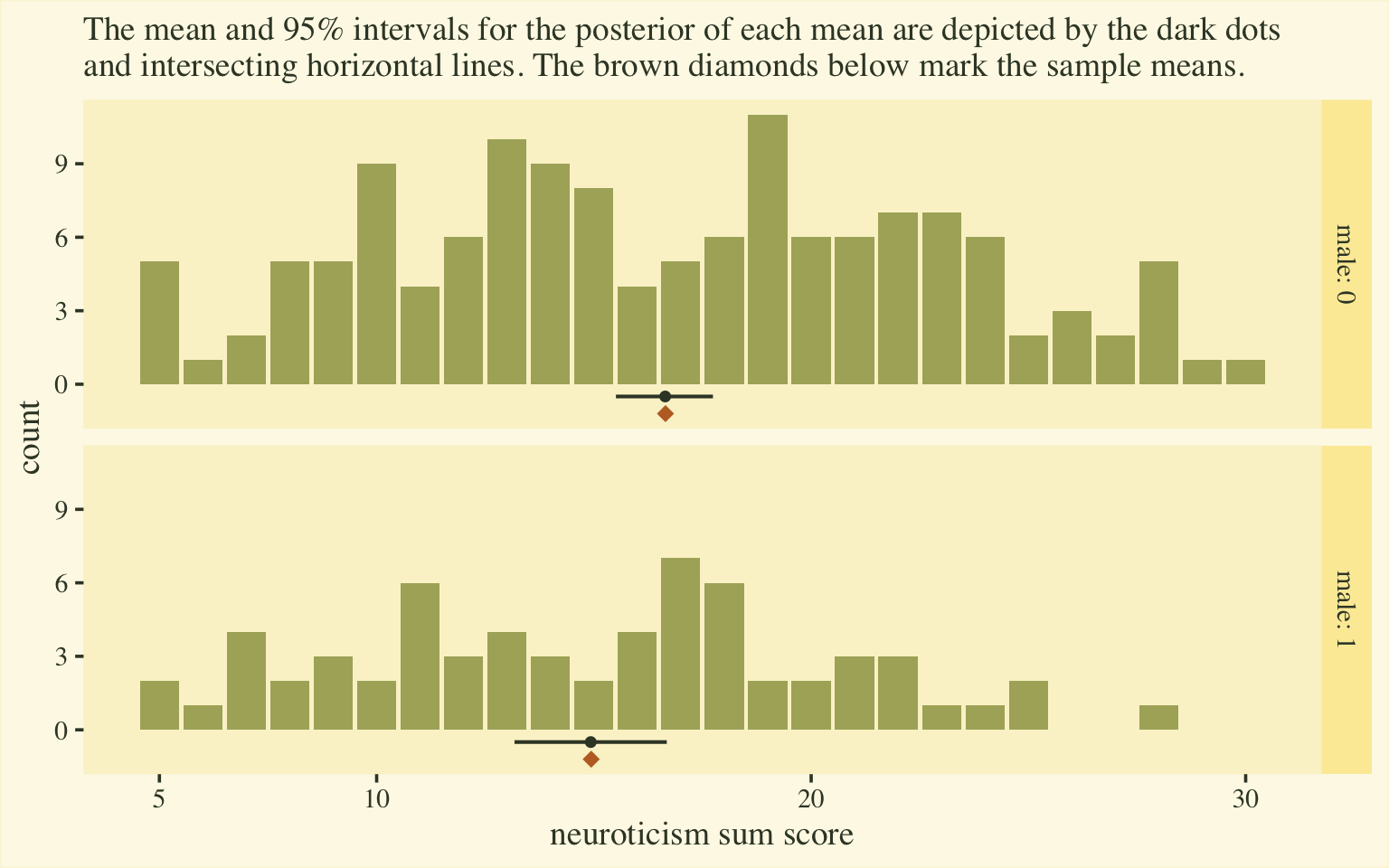
Happily, this time the posterior distributions for the sum-score means matched up nicely with the sample statistics. Now we have a sense of how to convert out posterior summaries into a sum-score metric, let’s explore effect sizes.

Unstandardized mean differences.

Probably the easiest way to express the sum-score difference between males and females with with an standardized mean difference.

d %>% 
  distinct(item, male) %>% 
  add_epred_draws(fit8, re_formula = ~ (1 | item)) %>% 
  mutate(product = as.double(.category) * .epred) %>% 
  # this line has been changed
  group_by(male, .draw) %>% 
  summarise(sum_score_mean = sum(product)) %>% 
  pivot_wider(names_from = male, values_from = sum_score_mean) %>% 
  mutate(d = `1` - `0`) %>% 
  
  ggplot(aes(x = d)) +
  stat_halfeye(.width = .95, fill = npp[14], color = npp[1]) +
  scale_y_continuous(NULL, breaks = NULL) +
  labs(title = "Neuroticism sum score effect size",
       x = "male - female (unstandardized mean difference)")

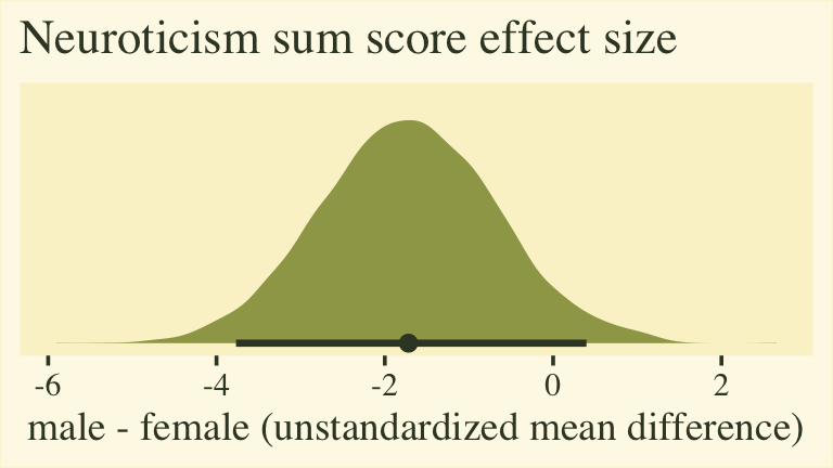
The plot shows that for the 5-to-30-point neuroticism sum score, males average about 2 points lower than females. To the extent this 5-item scale is widely used and understood by contemporary personality researchers, this might be a meaningful way to present the results. However, members of any audience unaccustomed to this five-item scale may find themselves wondering how impressed they should feel. This is the downfall of presenting an unstandardized mean difference for a scale with an arbitrary and idiosyncratic metric.

Standardized mean differences.

I’m generally a big fan of standardized mean differences, the most common of which are variants of Cohen’s \(d\). People report Cohen’s \(d\)’s for sum score data all the time. However, I don’t think that’s wise, here. If you look back into Cohen’s ( 1988) text, he introduced \(d\) as an effect size for two group means, based on data drawn from populations with normally distributed data. He made this clear in the first couple pages of Chapter 2, The t test for means. On page 19, for example: “The tables have been designed to render very simple the procedure for power analysis in the case where two samples, each of n cases, have been randomly and independently drawn from normal populations” (emphasis in the original). A little further down on the same page: “In the formal development of the t distribution for the difference between two independent means, the assumption is made that the populations sampled are normally distributed and that they are of homogeneous (i.e., equal) variance” (emphasis in the original). Then on the very next page, Cohen introduced his \(d\) effect size for data of this kind.

Here’s the issue: Sum-score data aren’t really normally distributed. There are a lot of ways to characterize Gaussian data. They’re continuous, unimodal, symmetric, bell-shaped, and not near any lower or upper boundaries¹. Given our finite sample size, it’s hard to determine how unimodal, symmetric, or bell-shaped the neuroticism sum scores might look in the population². But we know for sure that these sum-score data are not truly continuous and they have well-defined lower and upper boundaries. In fact, these characteristics are part of the reason we analyzed the data with a cumulative probit model to begin with. So if you are going to go to the trouble of analyzing your ordinal data with a cumulative probit model, I recommend you express the results with an effect size that was not explicitly designed for Gaussian data.

In conclusion, I think Cohen’s \(d\)’s are a bad fit for Likert-type items fit with cumulative probit models.

POMP differences.

Given how we just spent a section discrediting Cohen’s \(d\)’s for sum-score data, it’s satisfying that Patricia Cohen, Jacob Cohen, and colleagues ( 1999) are also the group who have provided us with a slick alternative. We can express our mean differences in a POMP-score metric. The acronym POMP stands for the percent of maximum possible. Say you have some score variable \(y\), which varies across \(i\) cases, and has a clear lower and upper limit. You can convert those data into a POMP metric with the formula

$$ \text{POMP}_i = \frac{y_i - \min(y_i)}{\max(y_i) - \min(y_i)} \times 100. $$

Here’s what that transformation would look like for our neuroticism sum-score values.

tibble(sum_score = 5:30) %>% 
  mutate(POMP = (sum_score - min(sum_score)) / (max(sum_score) - min(sum_score)) * 100) %>% 

  ggplot(aes(x = sum_score, y = POMP, label = POMP)) +
  geom_col(width = .75, color = npp[17], fill = npp[17]) +
  geom_text(nudge_y = 2, size = 2.75) +
  scale_x_continuous("neuroticism sum score", breaks = c(1, 2, 4, 6) * 5)

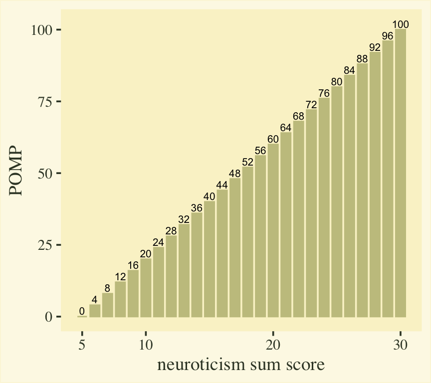
However, our strategy will not be to transform the neuroticism sum-score data, itself. Rather, we will transform the model-based means into the POMP metric, will will put our group contrasts into a POMP difference metric.

# define the min and max values
sum_score_min <- 5
sum_score_max <- 30

# start the same as before
pomp <- d %>% 
  distinct(item, male) %>% 
  add_epred_draws(fit8, re_formula = ~ (1 | item)) %>% 
  mutate(product = as.double(.category) * .epred,
         sex     = ifelse(male == 0, "female", "male")) %>% 
  group_by(sex, .draw) %>% 
  summarise(sum_score_mean = sum(product)) %>% 
  # compute the POMP scores
  mutate(pomp = (sum_score_mean - sum_score_min) / (sum_score_max - sum_score_min) * 100) %>% 
  # wrangle
  select(-sum_score_mean) %>% 
  pivot_wider(names_from = sex, values_from = pomp) %>% 
  mutate(`male - female` = male - female) %>% 
  pivot_longer(-.draw, values_to = "pomp") 

# plot
pomp %>% 
  ggplot(aes(x = pomp)) +
  stat_halfeye(point_interval = mean_qi, .width = .95, normalize = "panels",
               fill = npp[14], color = npp[1]) +
  scale_y_continuous(NULL, breaks = NULL) +
  labs(title = "Neuroticism sum score effect size",
       x = "percent of maximum possible (POMP)") +
  facet_wrap(~ name, scales = "free")

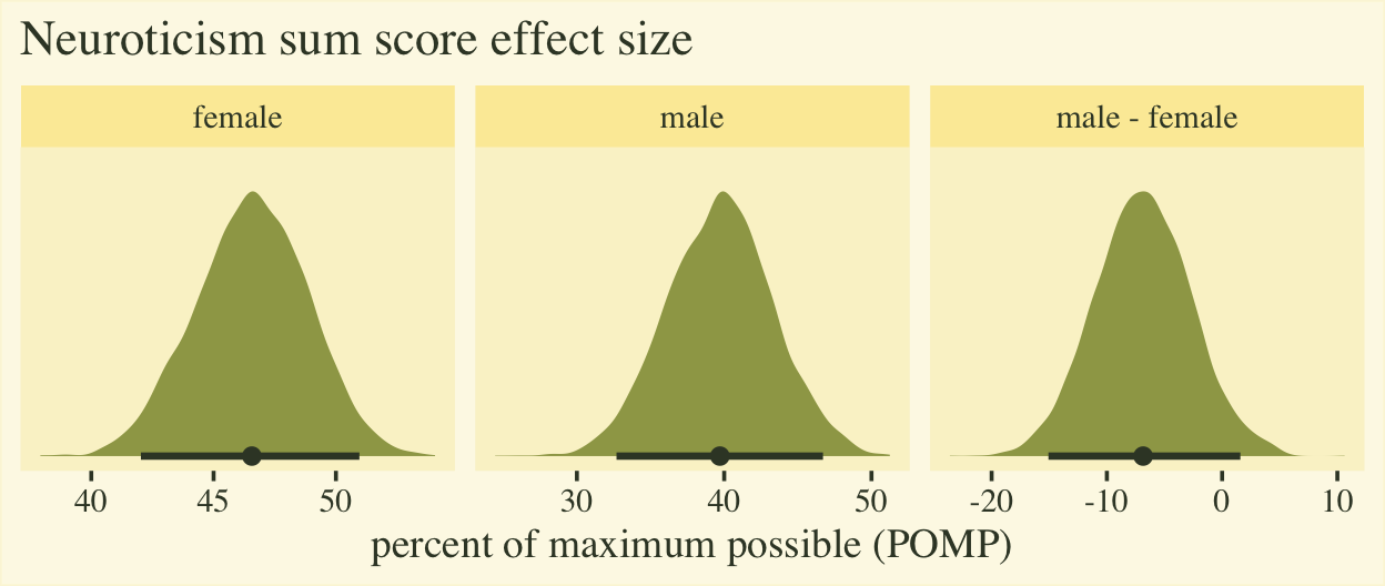
The plot shows the average scores for both males and females are a little below the middle of the full range of the neuroticism sum-score range, which bodes well from a psychometric perspective. The right panel clarifies the mean for males is about 7% lower than the mean for females, plus or minus 8%. To my mind, a POMP difference of 7% is large enough to take note.

If you’re curious, here are the numeric summaries.

pomp %>% 
  group_by(name) %>% 
  mean_qi(pomp) %>% 
  mutate_if(is.double, round, digits = 1)

## # A tibble: 3 × 7
##   name           pomp .lower .upper .width .point .interval
##   <chr>         <dbl>  <dbl>  <dbl>  <dbl> <chr>  <chr>    
## 1 female         46.6   42     51      0.9 mean   qi       
## 2 male           39.7   32.7   46.7    0.9 mean   qi       
## 3 male - female  -6.9  -15.1    1.6    0.9 mean   qi

POMP scores are handy, but they aren’t nearly as popular as unstandardized mean differences or Cohen’s \(d\)’s. I’m just warming up to them, myself. If you’d like more examples of how POMP scoring can look in applied research, check out Goodman et al. ( 2021) or Popescu et al. ( 2022)³.

Wrap it up

Okay friends, in this post we

• practiced analyzing several Likert-type items with a multilevel distributional Bayesian cumulative probit model,
• used the tidybayes::add_epred_draws() function to help compute conditional means for the items,
• extended that approach to compute conditional means for the sum score, and
• discussed three ways to express sum-score contrasts as effect sizes.

This topic is pushing the edges of my competence. If you have insights to add, chime in on twitter.

New blog up!https://t.co/UxZjhl2PVC

This is a follow-up to a post from a few months ago. Here we explore how to compute sum-score level effect sizes from Bayesian cumulative probit models fit to item-level data. In the end, I recommend @bmwiernik's beloved POMP scores.#brms https://t.co/HZ4BcBNnbi

— Solomon Kurz (@SolomonKurz) July 19, 2022

Happy modeling, friends.

Session info

sessionInfo()

## R version 4.2.0 (2022-04-22)
## Platform: x86_64-apple-darwin17.0 (64-bit)
## Running under: macOS Big Sur/Monterey 10.16
## 
## Matrix products: default
## BLAS:   /Library/Frameworks/R.framework/Versions/4.2/Resources/lib/libRblas.0.dylib
## LAPACK: /Library/Frameworks/R.framework/Versions/4.2/Resources/lib/libRlapack.dylib
## 
## locale:
## [1] en_US.UTF-8/en_US.UTF-8/en_US.UTF-8/C/en_US.UTF-8/en_US.UTF-8
## 
## attached base packages:
## [1] stats     graphics  grDevices utils     datasets  methods   base     
## 
## other attached packages:
##  [1] tidybayes_3.0.2 brms_2.18.0     Rcpp_1.0.9      forcats_0.5.1   stringr_1.4.1   dplyr_1.0.10    purrr_0.3.4    
##  [8] readr_2.1.2     tidyr_1.2.1     tibble_3.1.8    ggplot2_3.4.0   tidyverse_1.3.2
## 
## loaded via a namespace (and not attached):
##   [1] readxl_1.4.1           backports_1.4.1        plyr_1.8.7             igraph_1.3.4           svUnit_1.0.6          
##   [6] splines_4.2.0          crosstalk_1.2.0        TH.data_1.1-1          rstantools_2.2.0       inline_0.3.19         
##  [11] digest_0.6.30          htmltools_0.5.3        fansi_1.0.3            magrittr_2.0.3         checkmate_2.1.0       
##  [16] googlesheets4_1.0.1    tzdb_0.3.0             modelr_0.1.8           RcppParallel_5.1.5     matrixStats_0.62.0    
##  [21] xts_0.12.1             sandwich_3.0-2         prettyunits_1.1.1      colorspace_2.0-3       rvest_1.0.2           
##  [26] ggdist_3.2.0           haven_2.5.1            xfun_0.35              callr_3.7.3            crayon_1.5.2          
##  [31] jsonlite_1.8.3         lme4_1.1-31            survival_3.4-0         zoo_1.8-10             glue_1.6.2            
##  [36] gtable_0.3.1           gargle_1.2.0           emmeans_1.8.0          distributional_0.3.1   pkgbuild_1.3.1        
##  [41] rstan_2.21.7           abind_1.4-5            scales_1.2.1           mvtnorm_1.1-3          DBI_1.1.3             
##  [46] miniUI_0.1.1.1         xtable_1.8-4           stats4_4.2.0           StanHeaders_2.21.0-7   DT_0.24               
##  [51] htmlwidgets_1.5.4      httr_1.4.4             threejs_0.3.3          arrayhelpers_1.1-0     posterior_1.3.1       
##  [56] ellipsis_0.3.2         pkgconfig_2.0.3        loo_2.5.1              farver_2.1.1           sass_0.4.2            
##  [61] dbplyr_2.2.1           utf8_1.2.2             labeling_0.4.2         tidyselect_1.1.2       rlang_1.0.6           
##  [66] reshape2_1.4.4         later_1.3.0            munsell_0.5.0          cellranger_1.1.0       tools_4.2.0           
##  [71] cachem_1.0.6           cli_3.4.1              generics_0.1.3         broom_1.0.1            ggridges_0.5.3        
##  [76] evaluate_0.18          fastmap_1.1.0          yaml_2.3.5             processx_3.8.0         knitr_1.40            
##  [81] fs_1.5.2               nlme_3.1-159           mime_0.12              projpred_2.2.1         xml2_1.3.3            
##  [86] compiler_4.2.0         bayesplot_1.9.0        shinythemes_1.2.0      rstudioapi_0.13        gamm4_0.2-6           
##  [91] reprex_2.0.2           bslib_0.4.0            stringi_1.7.8          highr_0.9              ps_1.7.2              
##  [96] blogdown_1.15          Brobdingnag_1.2-8      NatParksPalettes_0.1.0 lattice_0.20-45        Matrix_1.4-1          
## [101] psych_2.2.5            nloptr_2.0.3           markdown_1.1           shinyjs_2.1.0          tensorA_0.36.2        
## [106] vctrs_0.5.0            pillar_1.8.1           lifecycle_1.0.3        jquerylib_0.1.4        bridgesampling_1.1-2  
## [111] estimability_1.4.1     httpuv_1.6.5           R6_2.5.1               bookdown_0.28          promises_1.2.0.1      
## [116] gridExtra_2.3          codetools_0.2-18       boot_1.3-28            colourpicker_1.1.1     MASS_7.3-58.1         
## [121] gtools_3.9.3           assertthat_0.2.1       withr_2.5.0            mnormt_2.1.0           shinystan_2.6.0       
## [126] multcomp_1.4-20        mgcv_1.8-40            parallel_4.2.0         hms_1.1.1              grid_4.2.0            
## [131] coda_0.19-4            minqa_1.2.5            rmarkdown_2.16         googledrive_2.0.0      shiny_1.7.2           
## [136] lubridate_1.8.0        base64enc_0.1-3        dygraphs_1.1.1.6

References

Blake, K. S. (2022). NatParksPalettes: Color palette package inspired by national parks. [Manual]. https://github.com/kevinsblake/NatParksPalettes
Bürkner, P.-C. (2020). Bayesian item response modeling in R with brms and Stan. http://arxiv.org/abs/1905.09501
Bürkner, P.-C. (2017). brms: An R package for Bayesian multilevel models using Stan. Journal of Statistical Software, 80(1), 1–28. https://doi.org/10.18637/jss.v080.i01
Bürkner, P.-C. (2018). Advanced Bayesian multilevel modeling with the R package brms. The R Journal, 10(1), 395–411. https://doi.org/10.32614/RJ-2018-017
Bürkner, P.-C. (2022). brms: Bayesian regression models using ’Stan’. https://CRAN.R-project.org/package=brms
Bürkner, P.-C., & Vuorre, M. (2019). Ordinal regression models in psychology: A tutorial. Advances in Methods and Practices in Psychological Science, 2(1), 77–101. https://doi.org/10.1177/2515245918823199
Cohen, J. (1988). Statistical power analysis for the behavioral sciences. L. Erlbaum Associates. https://www.worldcat.org/title/statistical-power-analysis-for-the-behavioral-sciences/oclc/17877467
Cohen, P., Cohen, J., Aiken, L. S., & West, S. G. (1999). The problem of units and the circumstance for POMP. Multivariate Behavioral Research, 34(3), 315–346. https://doi.org/10.1207/S15327906MBR3403_2
Efron, B., & Morris, C. (1977). Stein’s paradox in statistics. Scientific American, 236(5), 119–127. https://doi.org/10.1038/scientificamerican0577-119
Goldberg, L. R. (1999). A broad-bandwidth, public domain, personality inventory measuring the lower-level facets of several five-factor models. In I. Mervielde, I. Deary, F. De Fruyt, & F. Ostendorf (Eds.), Personality psychology in Europe (Vol. 7, pp. 7–28). Tilburg University Press.
Goodman, F. R., Kelso, K. C., Wiernik, B. M., & Kashdan, T. B. (2021). Social comparisons and social anxiety in daily life: An experience-sampling approach. Journal of Abnormal Psychology, 130(5), 468–489. https://doi.org/10.1037/abn0000671
Kay, M. (2022). tidybayes: Tidy data and ’geoms’ for Bayesian models. https://CRAN.R-project.org/package=tidybayes
Popescu, T., Stahl, B., Wiernik, B. M., Haiduk, F., Zemanek, M., Helm, H., Matzinger, T., Beisteiner, R., & Fitch, T. W. (2022). Melodic Intonation Therapy for aphasia: A multi-level meta-analysis or randomized controlled trials and individual participant data. Annals of the New York Academy of Sciences. https://doi.org/10.1111/nyas.14848
R Core Team. (2022). R: A language and environment for statistical computing. R Foundation for Statistical Computing. https://www.R-project.org/
Revelle, W. (2022). psych: Procedures for psychological, psychometric, and personality research. https://CRAN.R-project.org/package=psych
Revelle, W., Wilt, J., & Rosenthal, A. (2010). Individual differences in cognition: New methods for examining the personality-cognition link. In A. Gruszka, G. Matthews, & B. Szymura (Eds.), Handbook of individual differences in cognition: Attention, memory and executive control (pp. 27–49). Springer.
Wickham, H. (2022). tidyverse: Easily install and load the ’tidyverse’. https://CRAN.R-project.org/package=tidyverse
Wickham, H., Averick, M., Bryan, J., Chang, W., McGowan, L. D., François, R., Grolemund, G., Hayes, A., Henry, L., Hester, J., Kuhn, M., Pedersen, T. L., Miller, E., Bache, S. M., Müller, K., Ooms, J., Robinson, D., Seidel, D. P., Spinu, V., … Yutani, H. (2019). Welcome to the tidyverse. Journal of Open Source Software, 4(43), 1686. https://doi.org/10.21105/joss.01686
-
Technically, proper Gaussian data range between
\(-\infty\)and\(\infty\). In the real world, researchers generally find it acceptable to use the Gaussian likelihood as long as the data distributions aren’t too close to a lower or upper boundary. What constitutes “too close” is up for debate, and probably has more to do with the pickiness of one’s peer reviewers than anything else. ↩︎ -
Okay, I’m getting a little lazy, here. If you recall, our
ddata are a random subset of the 2,800-rowbfidata from the psych package. If you compute the neuroticism sum score from the full data set, you can get a better sense of the population distribution. As it turns out, they’re unimodal, but not particularly symmetric or bell shaped. ↩︎ -
Both examples of POMP used in the wild are co-authored by the great Brenton Wiernik, who is the person who first introduced me to POMP scoring. ↩︎
- Posted on:
- July 18, 2022
- Length:
- 27 minute read, 5572 words