Notes on the Bayesian cumulative probit

What/why?

Prompted by a couple of my research projects, I’ve been fitting a lot of ordinal models, lately. Because of its nice interpretive properties, I’m fond of using the cumulative probit. Though I’ve written about cumulative logit ( Kurz, 2020b, sec. 11.1) and probit models ( Kurz, 2020a, Chapter 23) before, I still didn’t feel grounded enough to make rational decisions about priors and parameter interpretations. In this post, I have collected my recent notes and reformatted them into something of a tutorial on the Bayesian cumulative probit model. Using a single psychometric data set, we explore a variety of models, starting with the simplest single-level thresholds-only model and ending with a conditional multilevel distributional model.

Be warned: This isn’t exactly a tutorial for beginners to the cumulative probit. For introductions, see some of the references cited within.

Set it up

All code is in R ( R Core Team, 2022), with healthy doses of the tidyverse ( Wickham et al., 2019; Wickham, 2022) for data wrangling and plotting. All models are fit with brms ( Bürkner, 2017, 2018, 2022). In addition, there are a couple places where I make good use of the tidybayes package ( Kay, 2022).

Here we load the packages and adjust the global plotting theme.

# load
library(tidyverse)
library(brms)
library(tidybayes)

# adjust the global plotting theme
theme_set(
  theme_gray(base_size = 13,
             base_family = "Times") +
  theme(panel.grid = element_blank())
)

Our data will be a subset of the bfi data ( Revelle et al., 2010) from the psych package ( Revelle, 2022). Here we load, subset, and wrangle the data to suit our needs.

set.seed(1)

d <- psych::bfi %>% 
  mutate(male = ifelse(gender == 1, 1, 0),
         female = ifelse(gender == 2, 1, 0)) %>% 
  drop_na() %>% 
  slice_sample(n = 200) %>% 
  mutate(id = 1:n()) %>% 
  select(id, male, female, N1:N5) %>% 
  pivot_longer(N1:N5, names_to = "item", values_to = "rating")

# what is this?
glimpse(d)

## Rows: 1,000
## Columns: 5
## $ id     <int> 1, 1, 1, 1, 1, 2, 2, 2, 2, 2, 3, 3, 3, 3, 3, 4, 4, 4, 4, 4, 5, 5, 5, 5, 5, 6, 6, 6, 6, 6, 7, 7, 7, 7, 7…
## $ male   <dbl> 1, 1, 1, 1, 1, 1, 1, 1, 1, 1, 0, 0, 0, 0, 0, 1, 1, 1, 1, 1, 0, 0, 0, 0, 0, 0, 0, 0, 0, 0, 0, 0, 0, 0, 0…
## $ female <dbl> 0, 0, 0, 0, 0, 0, 0, 0, 0, 0, 1, 1, 1, 1, 1, 0, 0, 0, 0, 0, 1, 1, 1, 1, 1, 1, 1, 1, 1, 1, 1, 1, 1, 1, 1…
## $ item   <chr> "N1", "N2", "N3", "N4", "N5", "N1", "N2", "N3", "N4", "N5", "N1", "N2", "N3", "N4", "N5", "N1", "N2", "…
## $ rating <int> 2, 2, 1, 1, 1, 3, 3, 2, 3, 3, 4, 4, 4, 4, 2, 5, 3, 4, 6, 2, 1, 1, 3, 2, 2, 2, 4, 4, 1, 2, 1, 2, 4, 4, 1…

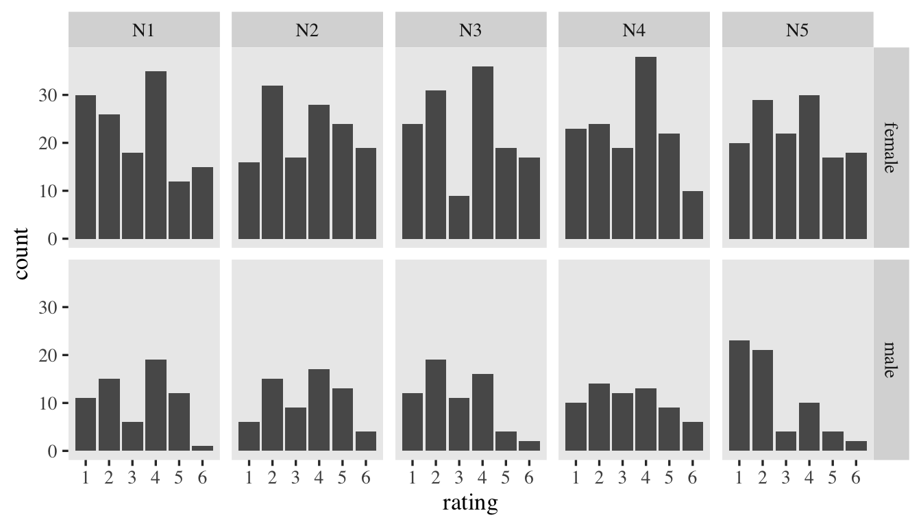
Our focal variables will be rating, which is a combination of the responses to the five questions in the Neuroticism scale of a version of the Big Five inventory ( Goldberg, 1999). Here’s a quick plot of the responses, by item and sex.

d %>% 
  mutate(sex = ifelse(male == 0, "female", "male")) %>% 
  
  ggplot(aes(x = rating)) +
  geom_bar() +
  scale_x_continuous(breaks = 1:6) +
  facet_grid(sex ~ item)

Basics of the ordered probit

I’ve had a difficult time understanding the notation used in these models. As McElreath ( 2015, p. 335) remarked, there are a lot of different notational approaches for describing these models. In this post, I’ll be using a blend of sensibilities from McElreath, Bürkner ( 2020), and Kruschke ( 2015). If you see flaws in my equations, do drop me a comment.

Given a Likert-type variable rating for which there are \(K + 1 = 6\) response options, you can model the relative probability of each ordinal category as

$$p(\text{rating} = k | \{ \tau_k \}) = f(\tau_k) - f(\tau_{k - 1}),$$

where \(\tau_k\) is the \(k^\text{th}\) threshold. On the left side of the equation, we stated the relative probabilities of the ordinal categories is conditional on our set of thresholds \(\{ \tau_k \}\), which is a shorthand for writing out \(\{k_1, k_2, k_3, k_4, k_5\}\). The \(f(\cdot)\) operator is a stand-in for some cumulative distribution function, which will allow us to map the cumulative probabilities onto an unbounded parameter space divided up by the \(K\) thresholds.

Because of its nice interpretative properties, I (and many others) like to use the cumulative standard normal distribution \(\Phi\) as our function \(f(\cdot)\), which means we can rewrite the equation as

$$p(\text{rating} = k | \{ \tau_k \}) = \Phi(\tau_k) - \Phi(\tau_{k - 1}),$$

where, to be explicit, the parameters for \(\Phi\) are fixed to \(\mu = 0\) and \(\sigma = 1\) for purposes of identification. However, if you wanted two write out the equation to explicitly include our fixed \(\mu\) and \(\sigma\) parameters, it could look like

$$p(\text{rating} = k | \{ \tau_k \}) = \Phi([\tau_k - \mu] / \sigma) - \Phi([\tau_{k - 1} - \mu] / \sigma).$$

But again, since those are both held constant as \(0\) and \(1\), respectively, substituting those values into the equation reduces to what it was, before. This is one of the nice things about starting off with the cumulative standard normal distribution.

Anyway, the thing to understand is that the area under the normal curve to the left of \(\tau_k\) is defined as \(\Phi(\tau_k)\), which is the cumulative probability mass for the \(k^\text{th}\) rating. The reason we have to subtract the area to the left of \(\Phi(\tau_{k - 1})\) from \(\Phi(\tau_k)\) is so we can isolate a relative probability from a cumulative probability. This applies in the same way for all the middle ratings–2 through 5 in our case. For the first and last ratings (1 and 6), we might add two virtual thresholds \(-\infty\) and \(\infty\), respectively. With the first rating, this means

$$ \begin{align*} p(\text{rating} = k | \{ \tau_k \}) & = \Phi(\tau_1) - \Phi({\color{blue}{\tau_0}}) \\ & = \Phi(\tau_1) - \Phi({\color{blue}{-\infty}} ) \\ & = \Phi(\tau_1) - \color{blue}0 \\ & = \Phi(\tau_1). \end{align*} $$

In a similar way, for the last rating we have

$$ \begin{align*} p(\text{rating} = k | \{ \tau_k \}) & = \Phi({\color{blue}{\tau_{K + 1}}} ) - \Phi(\tau_K) \\ & = \Phi({\color{blue}\infty} ) - \Phi(\tau_K) \\ & = {\color{blue}1} - \Phi(\tau_K). \end{align*} $$

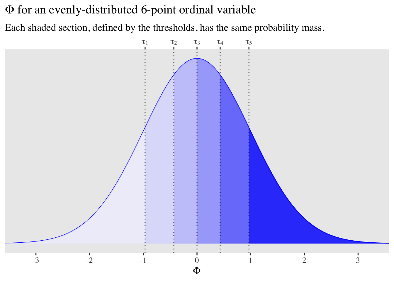
It might help to visualize this. Consider a case where we have a rating variable with 6 values (1 through 6), each with equal proportions, \(1 / 6 \approx .167.\) Here’s what that could look like mapped onto \(\Phi\).

tibble(z = seq(from = -3.75, to = 3.75, length.out = 1e3)) %>% 
  mutate(d = dnorm(x = z, mean = 0, sd = 1)) %>% 
  
  ggplot(aes(x = z, y = d)) +
  geom_line(color = "blue") +
  geom_area(aes(fill = z >= qnorm(p = 0 / 6)), alpha = 1/4) + 
  geom_area(aes(fill = z >= qnorm(p = 1 / 6)), alpha = 1/4) + 
  geom_area(aes(fill = z >= qnorm(p = 2 / 6)), alpha = 1/4) + 
  geom_area(aes(fill = z >= qnorm(p = 3 / 6)), alpha = 1/4) + 
  geom_area(aes(fill = z >= qnorm(p = 4 / 6)), alpha = 1/4) + 
  geom_area(aes(fill = z >= qnorm(p = 5 / 6)), alpha = 1/4) + 
  geom_vline(xintercept = qnorm(p = 1:5 / 6), linetype = 3) +
  scale_fill_manual(values = c("transparent", "blue"), breaks = NULL) +
  scale_x_continuous(expression(Phi), breaks = -3:3,
                     sec.axis = dup_axis(
    name = NULL,
    breaks = qnorm(p = 1:5 / 6),
    labels = parse(text = str_c("tau[", 1:5, "]"))
    )) +
  scale_y_continuous(NULL, breaks = NULL) +
  coord_cartesian(xlim = c(-3.25, 3.25)) +
  labs(title = expression(Phi*" for an evenly-distributed 6-point ordinal variable"),
       subtitle = "Each shaded section, defined by the thresholds, has the same probability mass.")

Here’s how you might compute some of those values within a tibble.

tibble(rating = 1:6) %>% 
  mutate(proportion = 1/6) %>% 
  mutate(cumulative_proportion = cumsum(proportion)) %>% 
  mutate(right_hand_threshold = qnorm(cumulative_proportion))

## # A tibble: 6 × 4
##   rating proportion cumulative_proportion right_hand_threshold
##    <int>      <dbl>                 <dbl>                <dbl>
## 1      1      0.167                 0.167               -0.967
## 2      2      0.167                 0.333               -0.431
## 3      3      0.167                 0.5                  0    
## 4      4      0.167                 0.667                0.431
## 5      5      0.167                 0.833                0.967
## 6      6      0.167                 1                  Inf

Alternatively, here’s how to use qnorm() within pnorm() to realize the various combinations of \(\Phi(\tau_k) - \Phi(\tau_{k - 1})\).

pnorm(q = qnorm(p = 1 / 6)) - pnorm(q = qnorm(p = 0 / 6))

## [1] 0.1666667

pnorm(q = qnorm(p = 2 / 6)) - pnorm(q = qnorm(p = 1 / 6))

## [1] 0.1666667

pnorm(q = qnorm(p = 3 / 6)) - pnorm(q = qnorm(p = 2 / 6))

## [1] 0.1666667

pnorm(q = qnorm(p = 4 / 6)) - pnorm(q = qnorm(p = 3 / 6))

## [1] 0.1666667

pnorm(q = qnorm(p = 5 / 6)) - pnorm(q = qnorm(p = 4 / 6))

## [1] 0.1666667

pnorm(q = qnorm(p = 6 / 6)) - pnorm(q = qnorm(p = 5 / 6))

## [1] 0.1666667

Models

For practice and building intuition, we’ll be fitting 8 models to the Neuroticism items. Starting simple and building up, they will be:

• fit1, the thresholds-only model;
• fit2, the single-level conditional mean model;
• fit3, the single-level conditional mean and dispersion model;
• fit4, the multilevel random participant-means model;
• fit5, the multilevel random participant- and item-level means model;
• fit6, the multilevel random participant- and item-level means model with varying thresholds;
• fit7, the multilevel unconditional distributional model; and
• fit8, the multilevel conditional distributional model.

I make no claim these titles are canonical. They just make sense to me.

Thresholds only.

Over the years, I’ve become fond of McElreath’s style of writing out models. His style usually looks something like

$$ \begin{align*} \text{criterion}_i & \sim \operatorname{Some likelihood}(\phi_i) \\ \text{some link function}(\phi_i) & = \alpha + \beta x_i \\ \alpha & \sim \text{< some prior >} \\ \beta & \sim \text{< some prior >}, \end{align*} $$

where \(\phi_i\) is a stand-in for the likelihood parameter(s). I’ve had a hard time applying this notation style to the cumulative probit model, so I’m going to detract a bit. Here’s my current attempt applied to the thresholds-only model:

$$ \begin{align*} p(\text{rating} = k | \{ \tau_k \}) & = \Phi(\tau_k) - \Phi(\tau_{k - 1}) \\ \tau_k & \sim \mathcal N(0, 2), \end{align*} $$

where the first line is the likelihood, which only contains the model parameters \(\tau_k\). The second line is a simple non-committal prior for the thresholds, which places \(95\%\) of the prior probability mass for each threshold between \(-4\) and \(4\). However, if we consider the plot above, we can come up with default prior that are a little less lazy. If we want our starting assumption to be a uniform distribution between our rating data, we could update the model to

$$ \begin{align*} p(\text{rating} = k | \{ \tau_k \}) & = \Phi(\tau_k) - \Phi(\tau_{k - 1}) \\ \tau_1 & \sim \mathcal N(-0.97, 1) \\ \tau_2 & \sim \mathcal N(-0.43, 1) \\ \tau_3 & \sim \mathcal N(0, 1) \\ \tau_4 & \sim \mathcal N(0.43, 1) \\ \tau_5 & \sim \mathcal N(0.97, 1), \end{align*} $$

where the priors are now all sequentially centered in different places in the \(\Phi\) space. Though it might initially seem bold to use \(1\) for the standard deviations on each, that’s still rather permissive when you consider the figure, above. I think you could easily justify using a \(0.5\) or so, instead.

Here’s how to fit the model with brms.

fit1 <- brm(
  data = d,
  family = cumulative(probit),
  rating ~ 1,
  prior = c(prior(normal(-0.97, 1), class = Intercept, coef = 1),
            prior(normal(-0.43, 1), class = Intercept, coef = 2),
            prior(normal( 0.00, 1), class = Intercept, coef = 3),
            prior(normal( 0.43, 1), class = Intercept, coef = 4),
            prior(normal( 0.97, 1), class = Intercept, coef = 5)),
  cores = 4,
  seed = 1,
  init_r = 0.2
)

You don’t necessarily have to adjust init_r, but my experience is these models often benefit from this adjustment.

Here’s the model summary.

print(fit1)

##  Family: cumulative 
##   Links: mu = probit; disc = identity 
## Formula: rating ~ 1 
##    Data: d (Number of observations: 1000) 
##   Draws: 4 chains, each with iter = 2000; warmup = 1000; thin = 1;
##          total post-warmup draws = 4000
## 
## Population-Level Effects: 
##              Estimate Est.Error l-95% CI u-95% CI Rhat Bulk_ESS Tail_ESS
## Intercept[1]    -0.94      0.05    -1.03    -0.85 1.00     3334     2650
## Intercept[2]    -0.25      0.04    -0.33    -0.17 1.00     5251     3510
## Intercept[3]     0.07      0.04    -0.00     0.15 1.00     4869     3513
## Intercept[4]     0.74      0.04     0.66     0.83 1.00     5449     3979
## Intercept[5]     1.32      0.05     1.21     1.43 1.00     5336     3509
## 
## Family Specific Parameters: 
##      Estimate Est.Error l-95% CI u-95% CI Rhat Bulk_ESS Tail_ESS
## disc     1.00      0.00     1.00     1.00   NA       NA       NA
## 
## Draws were sampled using sampling(NUTS). For each parameter, Bulk_ESS
## and Tail_ESS are effective sample size measures, and Rhat is the potential
## scale reduction factor on split chains (at convergence, Rhat = 1).

As Bürkner explained in his ( 2020) tutorial, the Intercept[k] rows are actually summarizing the \(\tau_k\) thresholds, not the \(\mu\) intercept for the underlying latent variable. That, recall, is fixed at \(0\) for identification purposes. Also, notice that the disc parameter is similarly held constant at \(1\) for identification.

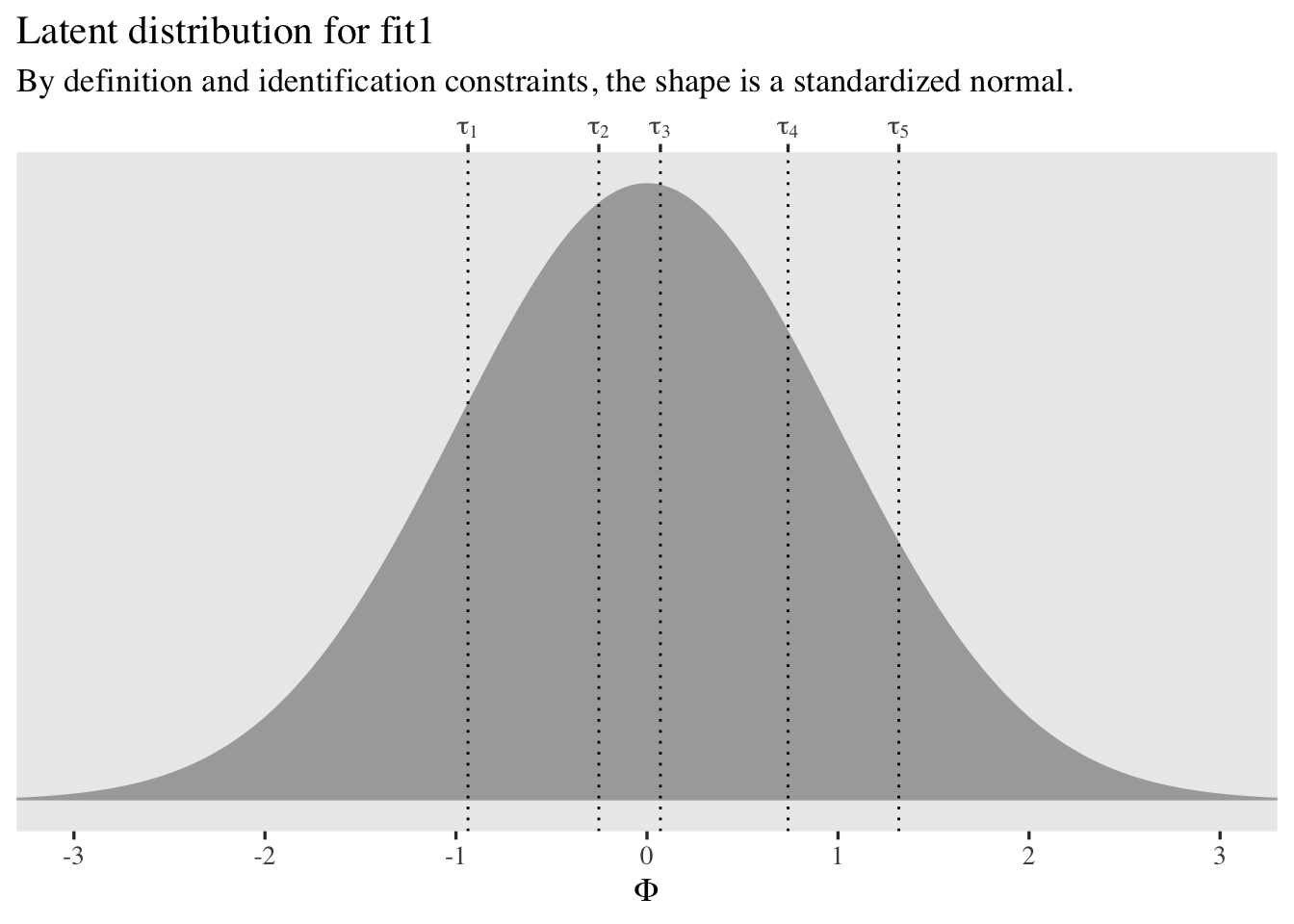
It might help to visualize the thresholds in a plot.

tibble(x = seq(from = -3.5, to = 3.5, length.out = 200)) %>% 
  mutate(d = dnorm(x = x)) %>% 
  
  ggplot(aes(x = x, y = d)) +
  geom_area(fill = "black", alpha = 1/3) +
  geom_vline(xintercept = fixef(fit1)[, 1], linetype = 3) +
  scale_x_continuous(expression(Phi), breaks = -3:3,
                     sec.axis = dup_axis(
    name = NULL,
    breaks = fixef(fit1)[, 1] %>% as.double(),
    labels = parse(text = str_c("tau[", 1:5, "]"))
    )) +
  scale_y_continuous(NULL, breaks = NULL) +
  coord_cartesian(xlim = c(-3, 3)) +
  labs(title = "Latent distribution for fit1",
       subtitle = "By definition and identification constraints, the shape is a standardized normal.")

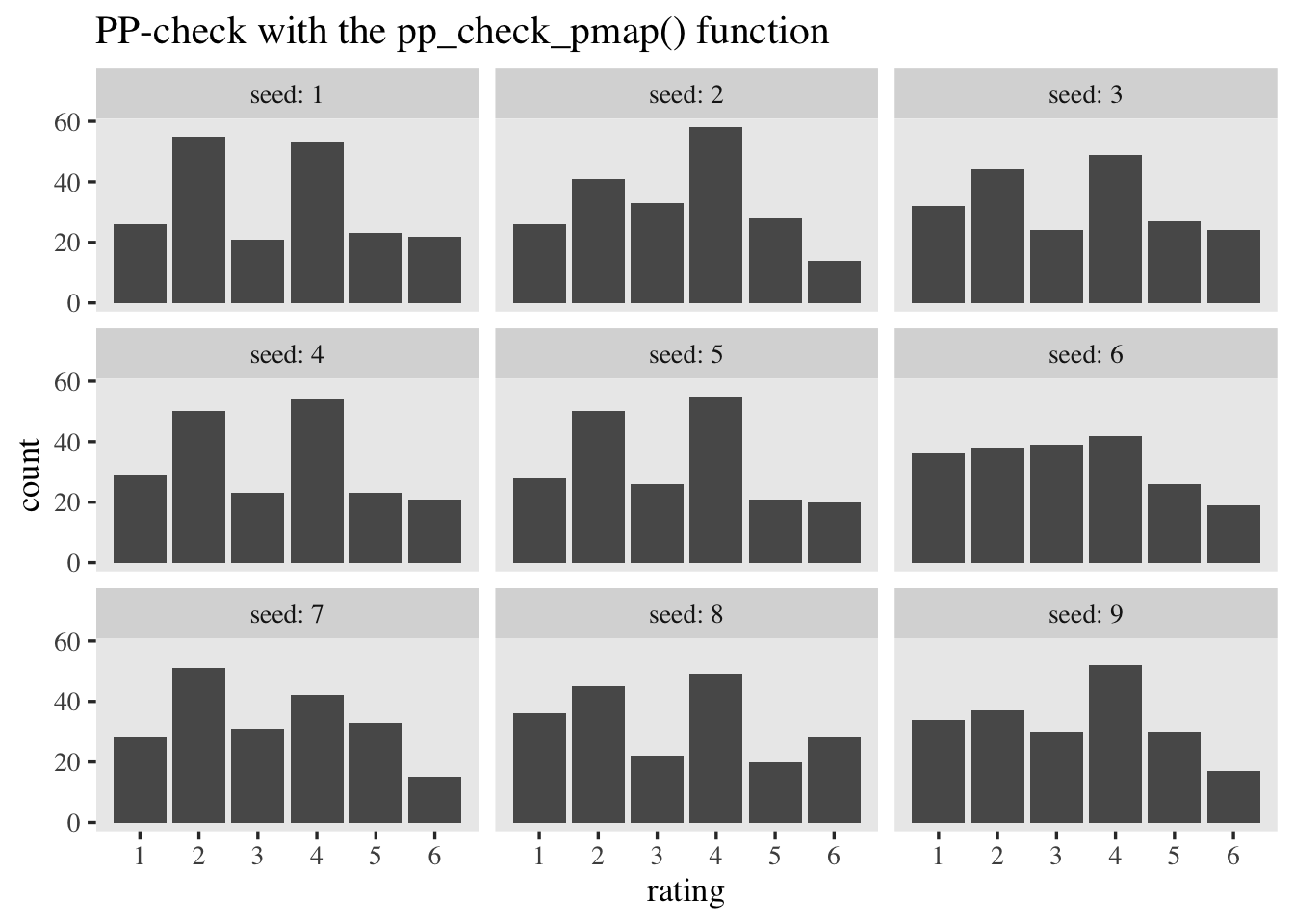
To get more practice working with the thresholds and how they relate to the actual rating data, it’ll help to to a couple posterior-predictive checks by hand. For our first version, we’ll make a custom function called pp_check_pmap(), which will make use of the pmap_dbl() function.

pp_check_pmap <- function(seed = 0) {
  
  set.seed(seed)
  
  as_draws_df(fit1) %>% 
    slice_sample(n = 200) %>% 
    select(starts_with("b_Intercept")) %>% 
    set_names(str_c("tau[", 1:5, "]")) %>% 
    mutate(p1 = pnorm(`tau[1]`),
           p2 = pnorm(`tau[2]`) - pnorm(`tau[1]`),
           p3 = pnorm(`tau[3]`) - pnorm(`tau[2]`),
           p4 = pnorm(`tau[4]`) - pnorm(`tau[3]`),
           p5 = pnorm(`tau[5]`) - pnorm(`tau[4]`),
           p6 = 1 - pnorm(`tau[5]`)) %>% 
    mutate(rating = pmap_dbl(.l = list(p1, p2, p3, p4, p5, p6),
                             .f = ~sample(
                               x = 1:6,
                               size = 1,
                               replace = TRUE,
                               prob = c(..1, ..2, ..3, ..4, ..5, ..6)
                             ))) %>% 
    select(rating)
  
}

Now use pp_check_pmap() to simulate \(9\) data sets resembling the original data.

tibble(seed = 1:9) %>% 
  mutate(sim = map(seed, pp_check_pmap)) %>% 
  unnest(sim) %>% 
  
  ggplot(aes(x = rating)) +
  geom_bar() +
  scale_x_continuous(breaks = 1:6) +
  ggtitle("PP-check with the pp_check_pmap() function") +
  facet_wrap(~ seed, labeller = label_both)

We can gain more insights into the model by using a different approach to computing the rating probabilities. This time, we’ll use an approach that leverages the case_when() function. We’ll wrap the approach in a custom function called pp_check_case_when().

pp_check_case_when <- function(seed = 0) {
  
  set.seed(seed)
  
  as_draws_df(fit1) %>% 
    slice_sample(n = 200) %>% 
    select(starts_with("b_Intercept")) %>% 
    set_names(str_c("tau[", 1:5, "]")) %>% 
    mutate(Phi = rnorm(n = n(), mean = 0, sd = 1)) %>% 
    mutate(rating = case_when(
      Phi < `tau[1]` ~ 1,
      Phi >= `tau[1]` & Phi < `tau[2]`~ 2,
      Phi >= `tau[2]` & Phi < `tau[3]`~ 3,
      Phi >= `tau[3]` & Phi < `tau[4]`~ 4,
      Phi >= `tau[4]` & Phi < `tau[5]`~ 5,
      Phi >= `tau[5]` ~ 6
    )) %>% 
    select(rating)
  
}

Now use pp_check_pmap() to simulate \(9\) data sets resembling the original data.

tibble(seed = 1:9) %>% 
  mutate(sim = map(seed, pp_check_case_when)) %>% 
  unnest(sim) %>% 
  
  ggplot(aes(x = rating)) +
  geom_bar() +
  scale_x_continuous(breaks = 1:6) +
  ggtitle("PP-check with the pp_check_case_when() function") +
  facet_wrap(~ seed, labeller = label_both)

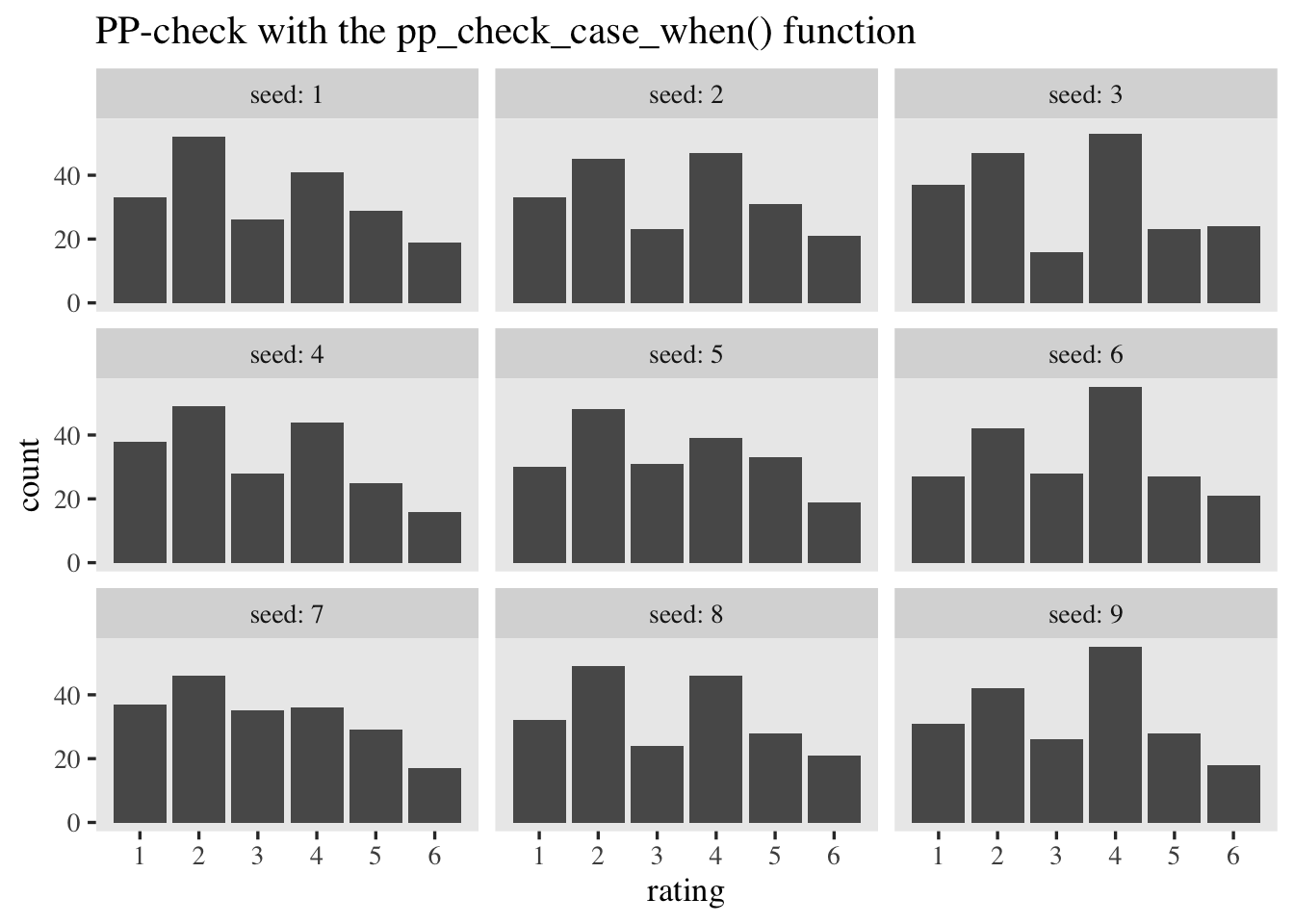
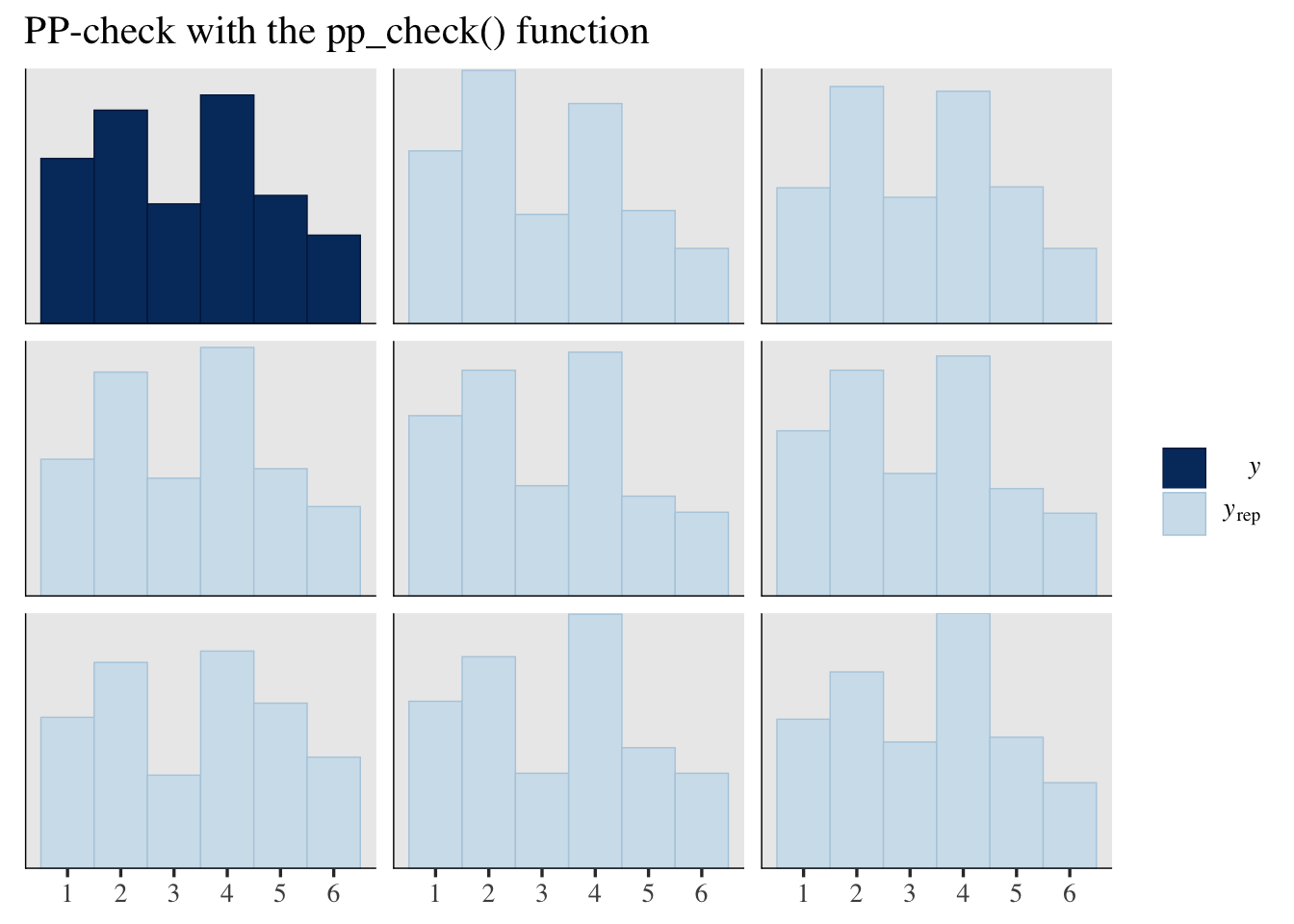
Both hand-done pp-checks returned similar results from those you can get with the pp_check() function.

pp_check(fit1, type = "hist", ndraws = 8, binwidth = 1) +
  scale_x_continuous(breaks = 1:6) +
  ggtitle("PP-check with the pp_check() function") 

Posterior predictive distributions are cool and all, but one of the most common sense questions a researcher would ask is How do I use the model to compute the mean of the data? When you have an ordinal model, the mean of the criterion variable is the sum of the \(p_k\) probabilities multiplied by the \(k\) values of the criterion. We might express this in an equation as

$$ \mathbb{E}(\text{rating}) = \sum_1^K p_k \times k, $$

where \(\mathbb{E}\) is the expectation operator (the model-based mean), \(p_k\) is the probability of the \(k^\text{th}\) ordinal value, and \(k\) is the actual ordinal value. The trick, here, is that because we are computing all the \(p_k\) values with MCMC and expressing those values as posterior distributions, we have to perform this operation within each of our MCMC draws. If we take cues from our pp_check_pmap(), above, we can compute this with our posterior draws like so.

as_draws_df(fit1) %>% 
  select(.draw, starts_with("b_Intercept")) %>% 
  set_names(".draw", str_c("tau[", 1:5, "]")) %>% 
  # compute the p_k distributions
  mutate(p1 = pnorm(`tau[1]`),
         p2 = pnorm(`tau[2]`) - pnorm(`tau[1]`),
         p3 = pnorm(`tau[3]`) - pnorm(`tau[2]`),
         p4 = pnorm(`tau[4]`) - pnorm(`tau[3]`),
         p5 = pnorm(`tau[5]`) - pnorm(`tau[4]`),
         p6 = 1 - pnorm(`tau[5]`)) %>% 
  # wrangle
  pivot_longer(starts_with("p"), values_to = "p") %>% 
  mutate(rating = str_extract(name, "\\d") %>% as.double()) %>% 
  # compute p_k * k
  mutate(`p * rating` = p * rating) %>% 
  # sum those values within each posterior draw
  group_by(.draw) %>% 
  summarise(mean_rating = sum(`p * rating`)) %>% 
  
  # plot!
  ggplot(aes(x = mean_rating, y = 0)) +
  stat_halfeye(.width = .95) +
  geom_vline(xintercept = mean(d$rating), linetype = 2) +
  scale_y_continuous(NULL, breaks = NULL) +
  labs(title = "The postrior for the mean of the rating values",
       subtitle = "The dashed vertical line marks off the sample mean. The posterior distribution is based on the\nsimple cumulative ordinal model fit1.",
       x = expression(mu[rating])) +
  xlim(2, 4)

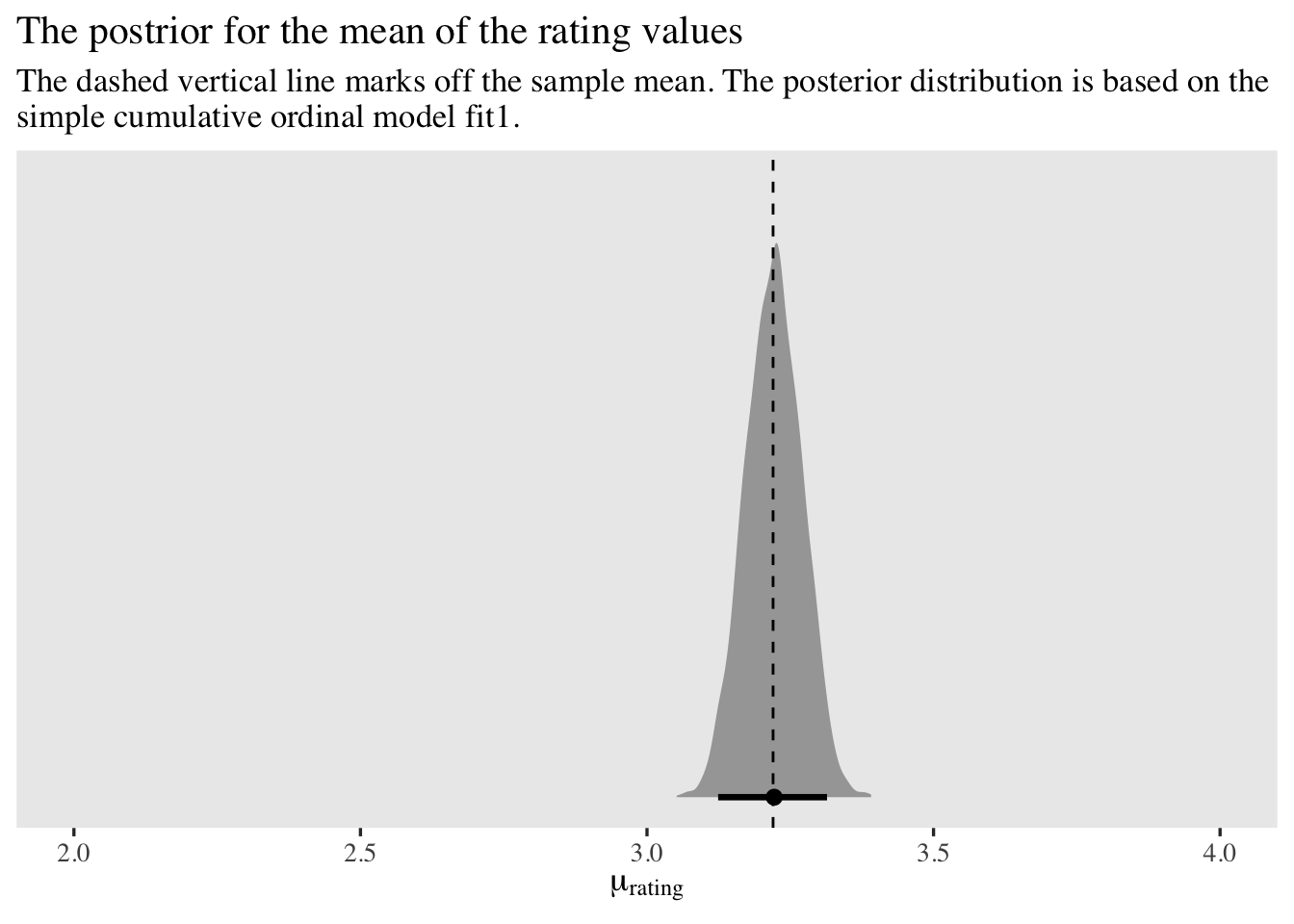
Our model did a great job finding the mean of the rating data.

Add a predictor.

If we would like to add a predictor, the most natural way is probably to explicitly add \(\mu\) in the likelihood and then attach a linear model to \(\mu_i\). This would look like

$$ \begin{align*} p(\text{rating} = k | \{ \tau_k \}, {\color{blue}{\mu_i}} ) & = \Phi(\tau_k {\color{blue}{- \mu_i}} ) - \Phi(\tau_{k - 1} {\color{blue}{- \mu_i}} ) \\ {\color{blue}{\mu_i}} & = {\color{blue}{\beta_0 + \sum_1^l \beta_l x_l}} \\ {\color{blue}{\beta_0}} & = {\color{blue}0} , \end{align*} $$

where \(\beta_0\) is the intercept for the latent mean and \(\sum_1^l \beta_l x_l\) is the additive effect of the full set of \(l\) predictor variables and their \(\beta_l\) coefficients. Now \(\beta_0\) is the parameter we set to zero for identification purposes. As before, the \(\sigma\) parameter will remain set to \(1\).

Since we are modeling a latent mean with a latent standard deviation of \(1\), this puts

• single continuous standardized predictors in a correlation metric and
• single dummy variables in a Cohen’s-$d$ metric.

As soon as you have multiple predictor variables in the mix, their metrics become increasingly difficult to interpret, but at least you can surmise that a partial correlation or a conditional Cohen’s \(d\) isn’t on a radically different metric from their univariable counterparts.

In the case of these data, our predictor of interest will be the dummy variable male. Thus, it makes sense to assign it a weakly-regularizing prior like \(\mathcal N(0, 1)\). Here’s the model formula:

$$ \begin{align*} p(\text{rating} = k | \{ \tau_k \}, \mu_i) & = \Phi(\tau_k - \mu_i) - \Phi(\tau_{k - 1} - \mu_i) \\ \mu_i & = \beta_1 \text{male}_i \\ \tau_1 & \sim \mathcal N(-0.97, 1) \\ \tau_2 & \sim \mathcal N(-0.43, 1) \\ \tau_3 & \sim \mathcal N(0, 1) \\ \tau_4 & \sim \mathcal N(0.43, 1) \\ \tau_5 & \sim \mathcal N(0.97, 1) \\ \beta_1 & \sim \mathcal N(0, 1), \end{align*} $$

where now the reference category is female. Here’s how to fit the model with brms.

# 49.33003 secs
fit2 <- brm(
  data = d,
  family = cumulative(probit),
  rating ~ 1 + male,
  prior = c(prior(normal(-0.97, 1), class = Intercept, coef = 1),
            prior(normal(-0.43, 1), class = Intercept, coef = 2),
            prior(normal( 0.00, 1), class = Intercept, coef = 3),
            prior(normal( 0.43, 1), class = Intercept, coef = 4),
            prior(normal( 0.97, 1), class = Intercept, coef = 5),
            prior(normal(0, 1), class = b)),
  cores = 4,
  seed = 1,
  init_r = 0.2
)

Check the summary.

print(fit2)

##  Family: cumulative 
##   Links: mu = probit; disc = identity 
## Formula: rating ~ 1 + male 
##    Data: d (Number of observations: 1000) 
##   Draws: 4 chains, each with iter = 2000; warmup = 1000; thin = 1;
##          total post-warmup draws = 4000
## 
## Population-Level Effects: 
##              Estimate Est.Error l-95% CI u-95% CI Rhat Bulk_ESS Tail_ESS
## Intercept[1]    -1.02      0.05    -1.12    -0.91 1.00     3167     3036
## Intercept[2]    -0.33      0.05    -0.42    -0.24 1.00     4809     3628
## Intercept[3]    -0.00      0.05    -0.09     0.09 1.00     4785     3571
## Intercept[4]     0.67      0.05     0.57     0.77 1.00     5309     3523
## Intercept[5]     1.25      0.06     1.13     1.37 1.00     5651     3799
## male            -0.22      0.07    -0.36    -0.09 1.00     5139     3154
## 
## Family Specific Parameters: 
##      Estimate Est.Error l-95% CI u-95% CI Rhat Bulk_ESS Tail_ESS
## disc     1.00      0.00     1.00     1.00   NA       NA       NA
## 
## Draws were sampled using sampling(NUTS). For each parameter, Bulk_ESS
## and Tail_ESS are effective sample size measures, and Rhat is the potential
## scale reduction factor on split chains (at convergence, Rhat = 1).

Since the \(\beta_1\) coefficient is a mean difference on the latent-$\Phi$ scale, it might be instructive to compare it to a Cohen’s \(d\) computed with the sample statistics. Here we compute the sample means, standard deviations, and sample sizes, by male.

# sample means
m_female <- d %>% filter(female == 1) %>% summarise(m = mean(rating)) %>% pull()
m_male   <- d %>% filter(male == 1)   %>% summarise(m = mean(rating)) %>% pull()

# sample standard deviations
s_female <- d %>% filter(female == 1) %>% summarise(s = sd(rating)) %>% pull()
s_male   <- d %>% filter(male == 1)   %>% summarise(s = sd(rating)) %>% pull()

# sample sizes
n_female <- d %>% filter(female == 1) %>% summarise(n = n()) %>% pull()
n_male   <- d %>% filter(male == 1)   %>% summarise(n = n()) %>% pull()

Now compute the pooled standard deviation.

s_pooled <- sqrt(((n_female - 1) * s_female^2 + (n_male - 1) * s_male^2) / (n_female + n_male - 2))

We’re finally ready to compute the sample Cohen’s \(d\).

(m_male - m_female) / s_pooled

## [1] -0.2167152

Compare that with the posterior mean and 95% CIs for our \(b_1\) parameter.

fixef(fit2)["male", -2]

##    Estimate        Q2.5       Q97.5 
## -0.22406785 -0.35812222 -0.08881928

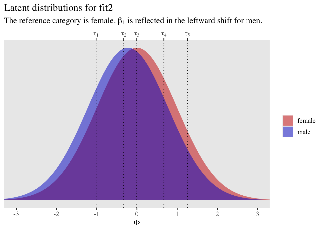
As with the first model, it might also be helpful to plot the latent distributions along with the thresholds.

tibble(male = 0:1,
       mu   = c(0, fixef(fit2)["male", 1])) %>% 
  expand(nesting(male, mu),
         x = seq(from = -3.5, to = 3.5, length.out = 200)) %>% 
  mutate(d   = dnorm(x, mean = mu, sd = 1),
         sex = ifelse(male == 0, "female", "male")) %>% 
  
  ggplot(aes(x = x, y = d, fill = sex)) +
  geom_area(alpha = 1/2, position = "identity") +
  geom_vline(xintercept = fixef(fit2)[1:5, 1], linetype = 3) +
  scale_fill_manual(NULL, values = c("red3", "blue3")) +
  scale_x_continuous(expression(Phi), breaks = -3:3,
                     sec.axis = dup_axis(
    name = NULL,
    breaks = fixef(fit2)[1:5, 1] %>% as.double(),
    labels = parse(text = str_c("tau[", 1:5, "]"))
    )) +
  scale_y_continuous(NULL, breaks = NULL) +
  coord_cartesian(xlim = c(-3, 3)) +
  labs(title = "Latent distributions for fit2",
       subtitle = expression("The reference category is female. "*beta[1]*" is reflected in the leftward shift for men."))

As before, we might also want to use our conditional fit2 to compute the population means for rating, by sex. We can extend our workflow from before by including the posterior draws for \(\beta_1\). Then when we use the pnorm() functions to compute the conditional probabilities, we’ll have to use \(\beta_1\) to adjust the values in the mean argument within pnorm() to account for the \(\mu_i = \beta_1 \text{male}_i\) portion of our statistical model.

as_draws_df(fit2) %>% 
  select(.draw, starts_with("b_")) %>% 
  set_names(".draw", str_c("tau[", 1:5, "]"), "beta[1]") %>% 
  # insert another copy of the data below
  bind_rows(., .) %>% 
  # add the two values for the dummy variable male
  mutate(male = rep(0:1, each = n() / 2)) %>% 
  # compute the p_k values conditional on the male dummy
  mutate(p1 = pnorm(`tau[1]`, mean = 0 + male * `beta[1]`),
         p2 = pnorm(`tau[2]`, mean = 0 + male * `beta[1]`) - pnorm(`tau[1]`, mean = 0 + male * `beta[1]`),
         p3 = pnorm(`tau[3]`, mean = 0 + male * `beta[1]`) - pnorm(`tau[2]`, mean = 0 + male * `beta[1]`),
         p4 = pnorm(`tau[4]`, mean = 0 + male * `beta[1]`) - pnorm(`tau[3]`, mean = 0 + male * `beta[1]`),
         p5 = pnorm(`tau[5]`, mean = 0 + male * `beta[1]`) - pnorm(`tau[4]`, mean = 0 + male * `beta[1]`),
         p6 = 1 - pnorm(`tau[5]`, mean = 0 + male * `beta[1]`)) %>%
  # wrangle
  pivot_longer(starts_with("p"), values_to = "p") %>% 
  mutate(rating = str_extract(name, "\\d") %>% as.double()) %>% 
  # compute p_k * k
  mutate(`p * rating` = p * rating) %>% 
  # sum those values within each posterior draw, by the male dummy
  group_by(.draw, male) %>% 
  summarise(mean_rating = sum(`p * rating`)) %>% 
  mutate(sex = ifelse(male == 0, "female", "male")) %>% 
  
  # the trick with and without fct_rev() helps order the axes, colors, and legend labels
  ggplot(aes(x = mean_rating, y = fct_rev(sex), fill = sex)) +
  stat_halfeye(.width = .95) +
  geom_vline(xintercept = m_male, linetype = 2, color = "blue3") +
  geom_vline(xintercept = m_female, linetype = 2, color = "red3") +
  scale_fill_manual(NULL, values = c(alpha("red3", 0.5), alpha("blue3", 0.5))) +
  labs(title = "The postrior for the mean of the rating values, by sex",
       subtitle = "The dashed vertical lines mark off the sample means, by sex. The posterior distributions\nare based on the simple conditional cumulative ordinal model fit2.",
       x = expression(mu[rating]),
       y = NULL) +
  xlim(2, 4) +
  theme(axis.text.y = element_text(hjust = 0))

By making the mean arguments within pnorm() conditional on our dummy male, we used our fit2 model to compute posteriors around the means of rating with great success.

Varying dispersion.

If we have reason to presume differences in latent standard deviations, we can explicitly add \(\sigma\) in the likelihood and then attach a linear model to \(\log(\sigma_i)\). As in other contexts, it’s generally a good idea to model \(\log(\sigma_i)\) instead of \(\sigma_i\) because the former will ensure the model will only predict positive values. This would look like

$$ \begin{align*} p(\text{rating} = k | \{ \tau_k \}, \mu_i, {\color{blue}{\sigma_i}} ) & = \Phi([\tau_k - \mu_i] {\color{blue}{/ \sigma_i}} ) - \Phi([\tau_{k - 1} - \mu_i] {\color{blue}{/ \sigma_i}} ) \\ \mu_i & = \beta_0 + \sum_1^l \beta_l x_l \\ {\color{blue}{\log(\sigma_i)}} & = {\color{blue}{\eta_0 + \sum_1^m \eta_m x_m}} \\ \beta_0 & = 0 \\ {\color{blue}{\eta_0}} & = {\color{blue}0} , \end{align*} $$

where \(\eta_0\) is the intercept for the logged latent standard deviation and \(\sum_1^m \eta_m x_m\) is the additive effect of the full set of \(m\) predictor variables and their \(\eta_m\) coefficients. Now \(\eta_0\) is set to zero for identification purposes. Recall that \(\exp(0) = 1\), which means that the default is still that \(\sigma_i = 1\) when all predictors are set to zero. With this model, it is possible the \(l\) and \(m\) predictor sets are the same. Here we differentiate between them just to make clear that they can differ, as needed.

A technical thing to keep in mind is that brms actually parameterizes cumulative probit models in terms of the discrimination parameter \(\alpha\), rather than \(\sigma\). Their relation is simple in that the one is the reciprocal of the other,

$$ \begin{align*} \sigma & = \frac{1}{\alpha}, \text{and} \\ \alpha & = \frac{1}{\sigma}. \end{align*} $$

It’s also the case that when you fit a model without a linear model attached to the discrimination parameter,

$$ \sigma = \frac{1}{\alpha} = \frac{1}{1} = 1. $$

However, things become more complicated when you want to model \(\alpha\). First, here’s the updated likelihood:

$$ \begin{align*} p(\text{rating} = k | \{ \tau_k \}, \mu_i, {\color{blue}{\alpha_i}} ) & = \Phi({\color{blue}{\alpha_i}} [\tau_k - \mu_i]) - \Phi( {\color{blue}{\alpha_i}} [\tau_{k - 1} - \mu_i]) \\ \mu_i & = \beta_0 + \sum_1^l \beta_l x_l \\ {\color{blue}{\log(\alpha_i)}} & = {\color{blue}{\eta_0 + \sum_1^m \eta_m x_m}} \\ \beta_0 & = 0 \\ \eta_0 & = 0. \end{align*} $$

If you want to convert \(\log(\alpha_i)\) to the \(\sigma\) metric, you need the transformation

$$ \sigma = \frac{1}{\exp(\log \alpha)}, $$

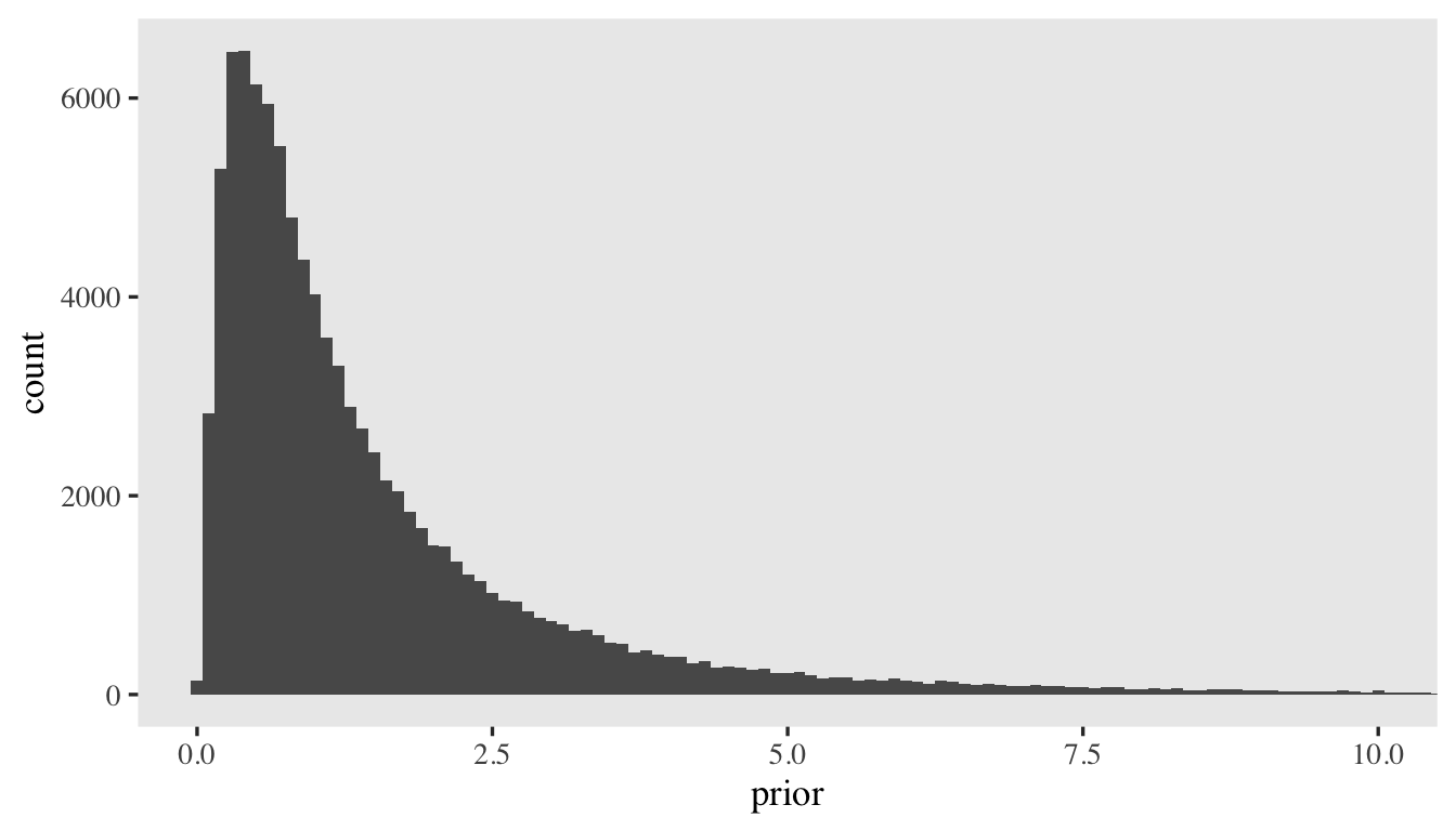
which puts the priors on the linear model for \(\log(\alpha_i)\) on an unfamiliar metric. As is often the case, something like \(\mathcal N(0, 1)\) is a good starting point. Here’s what it would look like if we simulated \(100{,}000\) draws from that prior and then converted them to the \(1 / \exp(\cdot)\) metric.

set.seed(1)

tibble(prior = rnorm(n = 1e5, mean = 0, sd = 1)) %>%
  mutate(prior = 1 / exp(prior)) %>%
  
  ggplot(aes(x = prior)) +
  geom_histogram(binwidth = 0.1) +
  # the right tail is very long
  coord_cartesian(xlim = c(0, 10))

We might extend this approach further to consider zero-centered normal priors with different values for the \(\sigma\) hyperparameter.

set.seed(1)

tibble(sigma_hyperparameter = 1:10 / 10) %>% 
  mutate(x = map(sigma_hyperparameter, ~ rnorm(n = 1e5, sd = .x))) %>% 
  unnest(x) %>% 
  mutate(x = 1 / exp(x)) %>% 
  group_by(sigma_hyperparameter) %>% 
  summarise(m = mean(x),
            mdn = median(x),
            s = sd(x),
            q2.5 = quantile(x, prob = .025),
            q97.5 = quantile(x, prob = .975)) %>% 
  mutate_all(round, digits = 2)

## # A tibble: 10 × 6
##    sigma_hyperparameter     m   mdn     s  q2.5 q97.5
##                   <dbl> <dbl> <dbl> <dbl> <dbl> <dbl>
##  1                  0.1  1.01     1  0.1   0.82  1.22
##  2                  0.2  1.02     1  0.21  0.67  1.48
##  3                  0.3  1.05     1  0.32  0.56  1.8 
##  4                  0.4  1.08     1  0.45  0.46  2.19
##  5                  0.5  1.13     1  0.6   0.38  2.66
##  6                  0.6  1.2      1  0.78  0.31  3.24
##  7                  0.7  1.28     1  1     0.25  3.93
##  8                  0.8  1.38     1  1.33  0.21  4.82
##  9                  0.9  1.5      1  1.72  0.17  5.85
## 10                  1    1.64     1  2.12  0.14  7.03

The median is always at \(1\), with varying levels of dispersion. But this doesn’t seem principled. It might be better to think in terms of how much change would be reasonable to see on \(\sigma\). In the present example, our sole predictor variable will be the dummy variable male. I’m not sure how much more or less variation we’d expect to see between the sexes on the Neuroticism ratings, but I’d be shocked if the standard deviation for one was more than twice the size of the other. Thus, since the reference category will be set to \(\sigma = 1\), we want a distribution where the bulk of the prior mass is set to half and twice that value.

sigma <- c(0.5, 1, 2)

Now convert those to \(\alpha\) values.

alpha <- 1 / sigma

Then, take the log of the \(\alpha\) values.

log(alpha)

## [1]  0.6931472  0.0000000 -0.6931472

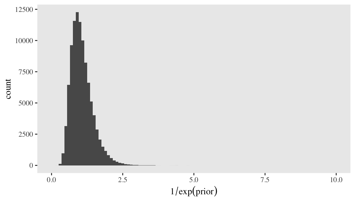
If \(\sigma_\text{men}\) were half the size of \(\sigma_\text{women}\), we’d expect \(\eta_1 = 0.693\). Similarly, if \(\sigma_\text{men}\) were twice the size of \(\sigma_\text{women}\), we’d expect \(\eta_1 = -0.693\). Thus the prior \(\eta_i \sim \mathcal N(0, 0.693 / 2 \approx 0.347)\) would put \(95 \%\) of the prior mass within the desired range.

We can compute that value with \(\log(2) / 2\), too.

log(2) / 2

## [1] 0.3465736

Here’s a histogram of what that would look like in the \(1 / \exp(\cdot)\) metric.

set.seed(1)

tibble(prior = rnorm(n = 1e5, mean = 0, sd = log(2) / 2)) %>%
  mutate(prior = 1 / exp(prior)) %>%
  
  ggplot(aes(x = prior)) +
  geom_histogram(binwidth = 0.1) +
  xlab(expression(1/exp(prior))) +
  coord_cartesian(xlim = c(0, 10))

With that all in mind, we can now update our model formula to:

$$ \begin{align*} p(\text{rating} = k | \{ \tau_k \}, \mu_i, \alpha_i) & = \Phi(\alpha_i[\tau_k - \mu_i]) - \Phi(\alpha_i[\tau_{k - 1} - \mu_i]) \\ \mu_i & = \beta_1 \text{male}_i \\ \log(\alpha_i) & = \eta_1 \text{male}_i\\ \tau_1 & \sim \mathcal N(-0.97, 1) \\ \tau_2 & \sim \mathcal N(-0.43, 1) \\ \tau_3 & \sim \mathcal N(0, 1) \\ \tau_4 & \sim \mathcal N(0.43, 1) \\ \tau_5 & \sim \mathcal N(0.97, 1) \\ \beta_1 & \sim \mathcal N(0, 1) \\ \eta_1 & \sim \mathcal N(0, 0.347). \end{align*} $$

Here’s how to fit the model with brms.

# 49.94408 secs
fit3 <- brm(
  data = d,
  family = cumulative(probit),
  bf(rating ~ 1 + male) +
    lf(disc ~ 0 + male,
       # this is really important
       cmc = FALSE),
  prior = c(prior(normal(-0.97, 1), class = Intercept, coef = 1),
            prior(normal(-0.43, 1), class = Intercept, coef = 2),
            prior(normal( 0.00, 1), class = Intercept, coef = 3),
            prior(normal( 0.43, 1), class = Intercept, coef = 4),
            prior(normal( 0.97, 1), class = Intercept, coef = 5),
            prior(normal(0, 1), class = b),
            # log(2) / 2 = 0.347
            prior(normal(0, log(2) / 2), class = b, dpar = disc)),
  cores = 4,
  seed = 1,
  init_r = 0.2
)

Note how we used the 0 + ... syntax in the first line in the lf() function and that set we set cmc = FALSE in the second line. As Bürkner noted in his ( 2020) tutorial, it’s critical that you do this when attaching a model to \(\log(\alpha_i)\). If you leave these bits out, you might find that you are no longer keeping the reference category for \(\log(\alpha_i)\) set to \(0\), which can wreak havoc on the model.

Anyway, check the summary.

print(fit3)

##  Family: cumulative 
##   Links: mu = probit; disc = log 
## Formula: rating ~ 1 + male 
##          disc ~ 0 + male
##    Data: d (Number of observations: 1000) 
##   Draws: 4 chains, each with iter = 2000; warmup = 1000; thin = 1;
##          total post-warmup draws = 4000
## 
## Population-Level Effects: 
##              Estimate Est.Error l-95% CI u-95% CI Rhat Bulk_ESS Tail_ESS
## Intercept[1]    -0.97      0.06    -1.08    -0.86 1.00     2359     2981
## Intercept[2]    -0.31      0.05    -0.41    -0.22 1.00     4558     3583
## Intercept[3]    -0.00      0.05    -0.09     0.09 1.00     5101     3616
## Intercept[4]     0.65      0.05     0.55     0.74 1.00     4746     3483
## Intercept[5]     1.22      0.06     1.10     1.33 1.00     4543     3337
## male            -0.20      0.07    -0.34    -0.08 1.00     4535     2831
## disc_male        0.12      0.06     0.00     0.24 1.00     2799     2612
## 
## Draws were sampled using sampling(NUTS). For each parameter, Bulk_ESS
## and Tail_ESS are effective sample size measures, and Rhat is the potential
## scale reduction factor on split chains (at convergence, Rhat = 1).

It can be challenging to interpret the disc_male coefficient directly. Keep in mind that larger values mean smaller relative values on the \(\sigma\) scale. Given how the reference value is \(0\), which equivalent to \(\sigma = 1\), this is the estimate of the latent standard deviation for men.

1 / exp(0 + fixef(fit3)["disc_male", -2])

##  Estimate      Q2.5     Q97.5 
## 0.8873625 0.9976675 0.7883039

Here are the two sample standard deviations.

s_female 

## [1] 1.616471

s_male

## [1] 1.491827

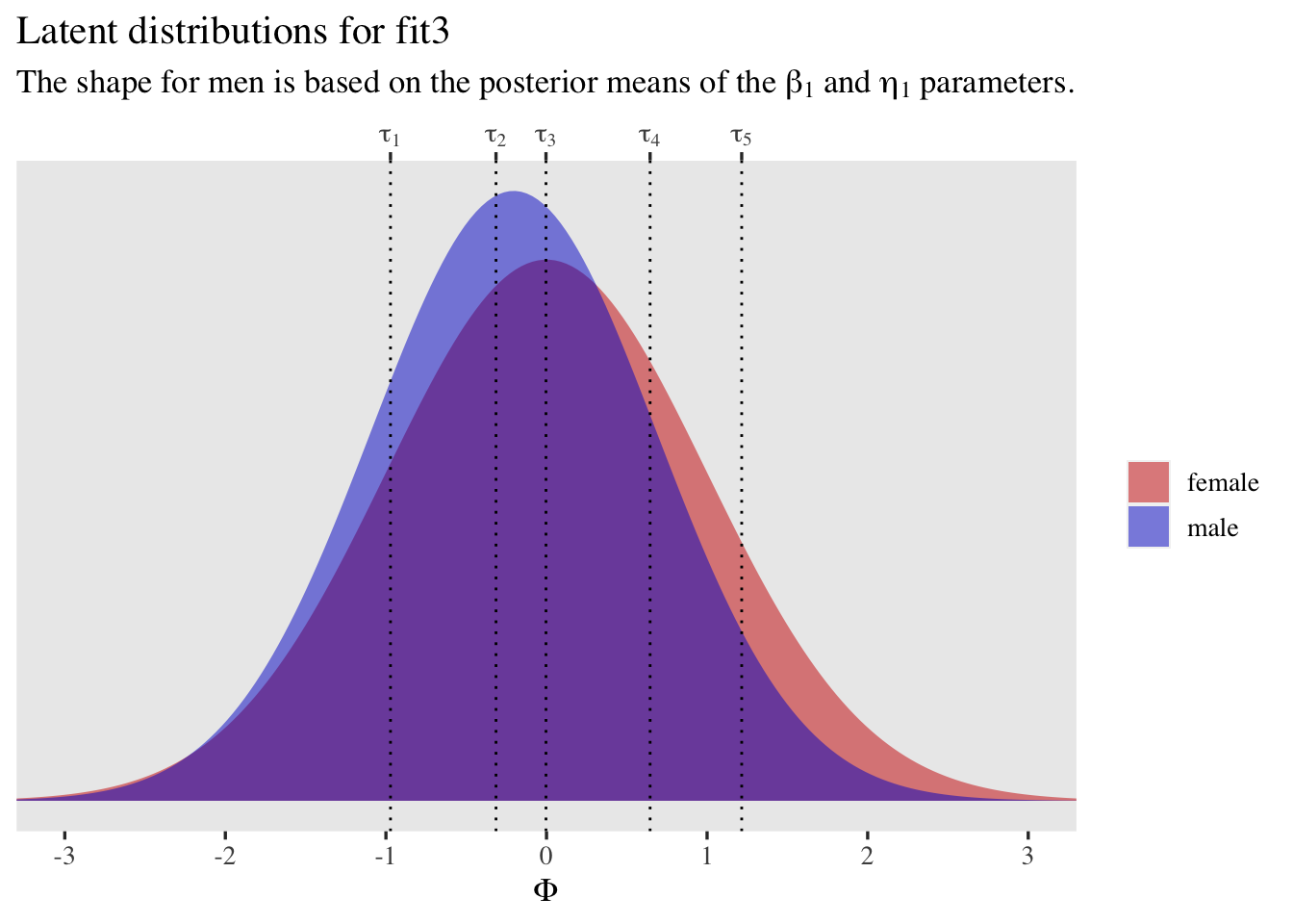
Once again, let’s plot.

tibble(male  = 0:1,
       mu    = c(0, fixef(fit3)["male", 1]),
       sigma = 1 / exp(c(0, fixef(fit3)["disc_male", 1]))) %>% 
  expand(nesting(male, mu, sigma),
         x = seq(from = -3.5, to = 3.5, length.out = 200)) %>% 
  mutate(d   = dnorm(x, mean = mu, sd = sigma),
         sex = ifelse(male == 0, "female", "male")) %>% 
  
  ggplot(aes(x = x, y = d, fill = sex)) +
  geom_area(alpha = 1/2, position = "identity") +
  geom_vline(xintercept = fixef(fit3)[1:5, 1], linetype = 3) +
  scale_fill_manual(NULL, values = c("red3", "blue3")) +
  scale_x_continuous(expression(Phi), breaks = -3:3,
                     sec.axis = dup_axis(
    name = NULL,
    breaks = fixef(fit3)[1:5, 1] %>% as.double(),
    labels = parse(text = str_c("tau[", 1:5, "]"))
    )) +
  scale_y_continuous(NULL, breaks = NULL) +
  labs(title = "Latent distributions for fit3",
       subtitle = expression("The shape for men is based on the posterior means of the "*beta[1]*" and "*eta[1]*" parameters.")) +
  coord_cartesian(xlim = c(-3, 3))

Note, however, that because this new model fit3 now has separate \(\sigma\) estimates by sex, the \(\beta_1\) parameter isn’t quite in a standardized-mean-difference metric, anymore. To get it back in to a \(d\) metric, we’ll have to use the full posterior distribution for \(\sigma_\text{female}\) and \(\sigma_\text{male}\) to compute a model-based pooled standard deviation, by which we can then standardize the \(\beta_1\) coefficient.

as_draws_df(fit3) %>% 
  mutate(sigma_f = 1,
         sigma_m = 1 / exp(b_disc_male)) %>%
  mutate(sigma_pooled = sqrt(((n_female - 1) * sigma_f^2 + (n_male - 1) * sigma_m^2) / (n_female + n_male - 2))) %>% 
  transmute(d = b_male / sigma_pooled) %>% 
  mean_qi(d) %>% 
  mutate_if(is.double, round, digits = 3)

## # A tibble: 1 × 6
##        d .lower .upper .width .point .interval
##    <dbl>  <dbl>  <dbl>  <dbl> <chr>  <chr>    
## 1 -0.212 -0.345  -0.08   0.95 mean   qi

Also, consider the variance metric. Given that the standard deviation squared is the variance, \(\sigma^2\), an increase of doubling the standard deviation is the same as quadrupling the variance.

2^2

## [1] 4

If you wanted to set up the model so that \(95\%\) of the prior probability allowed for a doubling of the variance, you’d need to set the upper range to the square root of \(2\).

sqrt(2)

## [1] 1.414214

Anyway, now that we’ve updated the model to account for differences in \(\sigma\), we might also want to update our workflow for computing the population means for rating. The trick is now the sd argument within the pnorm() function should be conditional on the values for males or females. Here’s one way how.

as_draws_df(fit3) %>% 
  # this also includes the column for b_disc_male
  select(.draw, starts_with("b_")) %>% 
  set_names(".draw", str_c("tau[", 1:5, "]"), "beta[1]", "eta[1]") %>% 
  bind_rows(., .) %>% 
  mutate(male = rep(0:1, each = n() / 2)) %>% 
  # compute the conditional mu and sigma values
  mutate(mu_i    = 0 + male * `beta[1]`,
         sigma_i = 1 / exp(0 + male * `eta[1]`)) %>%
  # compute the p_k values conditional on the male dummy and the mu_i and sigma_i values
  mutate(p1 = pnorm(`tau[1]`, mean = mu_i, sd = sigma_i),
         p2 = pnorm(`tau[2]`, mean = mu_i, sd = sigma_i) - pnorm(`tau[1]`, mean = mu_i, sd = sigma_i),
         p3 = pnorm(`tau[3]`, mean = mu_i, sd = sigma_i) - pnorm(`tau[2]`, mean = mu_i, sd = sigma_i),
         p4 = pnorm(`tau[4]`, mean = mu_i, sd = sigma_i) - pnorm(`tau[3]`, mean = mu_i, sd = sigma_i),
         p5 = pnorm(`tau[5]`, mean = mu_i, sd = sigma_i) - pnorm(`tau[4]`, mean = mu_i, sd = sigma_i),
         p6 = 1 - pnorm(`tau[5]`, mean = mu_i, sd = sigma_i)) %>%
  # the rest is now the same as before
  pivot_longer(starts_with("p"), values_to = "p") %>% 
  mutate(rating = str_extract(name, "\\d") %>% as.double()) %>% 
  mutate(`p * rating` = p * rating) %>% 
  group_by(.draw, male) %>% 
  summarise(mean_rating = sum(`p * rating`)) %>% 
  mutate(sex = ifelse(male == 0, "female", "male")) %>% 
  
  ggplot(aes(x = mean_rating, y = fct_rev(sex), fill = sex)) +
  stat_halfeye(.width = .95) +
  geom_vline(xintercept = m_male, linetype = 2, color = "blue3") +
  geom_vline(xintercept = m_female, linetype = 2, color = "red3") +
  scale_fill_manual(NULL, values = c(alpha("red3", 0.5), alpha("blue3", 0.5))) +
  labs(title = "The postrior for the mean of the rating values, by sex",
       subtitle = "The dashed vertical lines mark off the sample means, by sex. The posterior distributions\nare based on the simple conditional cumulative ordinal model fit3.",
       x = expression(mu[rating]),
       y = NULL) +
  xlim(2, 4) +
  theme(axis.text.y = element_text(hjust = 0))

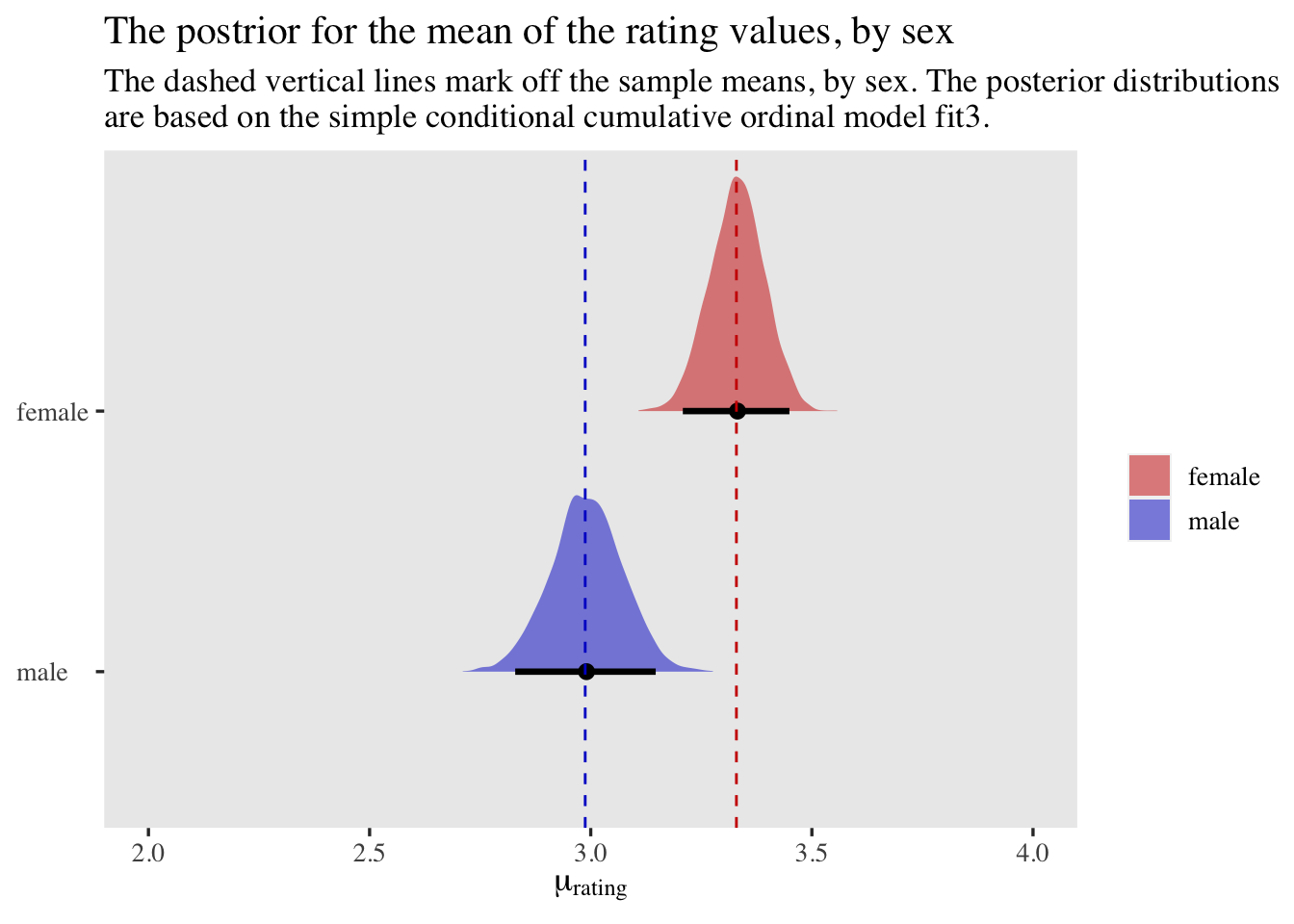
The results are very similar to those from above.

Randomly-varying latent means.

Up until now, we’ve been ignoring how this model has a multilevel structure. We have ratings nested within persons (id) and questions (item). Within cumulative probit models, the simplest way to account for that nesting is to add random intercepts to the latent mean, which will now be \(\mu_{ij}\) for the \(i^\text{th}\) person and the \(j^\text{th}\) question.

Starting slow, we’ll first just add random intercepts for the persons with the model

$$ \begin{align*} p(\text{rating} = k | \{ \tau_k \}, \mu_i) & = \Phi(\tau_k - \mu_i) - \Phi(\tau_{k - 1} - \mu_i) \\ \mu_i & = 0 + {\color{blue}{u_i}} \\ {\color{blue}{u_i}} & \sim {\color{blue}{\mathcal N(0, \sigma_u)}} \\ \tau_1 & \sim \mathcal N(-0.97, 1) \\ \tau_2 & \sim \mathcal N(-0.43, 1) \\ \tau_3 & \sim \mathcal N(0, 1) \\ \tau_4 & \sim \mathcal N(0.43, 1) \\ \tau_5 & \sim \mathcal N(0.97, 1) \\ {\color{blue}{\sigma_u}} & \sim {\color{blue}{\operatorname{Exponential}(1)}}, \end{align*} $$

where we’ve dropped the male predictor and the entire linear model for \(\log(\alpha_i)\) for the sake of simplicity. They’ll come back in a bit. Given the baseline fixed-effects portion of the model is still on the standardized-normal metric, the good old \(\operatorname{Exponential}(1)\) prior is a good choice for the level-2 standard deviation \(\sigma_u\). For more on the \(\operatorname{Exponential}(1)\) prior, see McElreath ( 2020).

Here’s how to fit the model with brms.

# 49.94408 secs
fit4 <- brm(
  data = d,
  family = cumulative(probit),
  rating ~ 1 + (1 | id),
  prior = c(prior(normal(-0.97, 1), class = Intercept, coef = 1),
            prior(normal(-0.43, 1), class = Intercept, coef = 2),
            prior(normal( 0.00, 1), class = Intercept, coef = 3),
            prior(normal( 0.43, 1), class = Intercept, coef = 4),
            prior(normal( 0.97, 1), class = Intercept, coef = 5),
            prior(exponential(1), class = sd)),
  cores = 4,
  seed = 1,
  init_r = 0.2
)

Check the summary.

print(fit4)

##  Family: cumulative 
##   Links: mu = probit; disc = identity 
## Formula: rating ~ 1 + (1 | id) 
##    Data: d (Number of observations: 1000) 
##   Draws: 4 chains, each with iter = 2000; warmup = 1000; thin = 1;
##          total post-warmup draws = 4000
## 
## Group-Level Effects: 
## ~id (Number of levels: 200) 
##               Estimate Est.Error l-95% CI u-95% CI Rhat Bulk_ESS Tail_ESS
## sd(Intercept)     1.03      0.07     0.90     1.18 1.00     1095     2370
## 
## Population-Level Effects: 
##              Estimate Est.Error l-95% CI u-95% CI Rhat Bulk_ESS Tail_ESS
## Intercept[1]    -1.33      0.10    -1.52    -1.15 1.00     1267     1809
## Intercept[2]    -0.37      0.09    -0.54    -0.21 1.00     1286     2043
## Intercept[3]     0.09      0.09    -0.08     0.25 1.00     1278     1982
## Intercept[4]     1.04      0.09     0.86     1.22 1.00     1369     2298
## Intercept[5]     1.86      0.10     1.66     2.07 1.00     1665     2743
## 
## Family Specific Parameters: 
##      Estimate Est.Error l-95% CI u-95% CI Rhat Bulk_ESS Tail_ESS
## disc     1.00      0.00     1.00     1.00   NA       NA       NA
## 
## Draws were sampled using sampling(NUTS). For each parameter, Bulk_ESS
## and Tail_ESS are effective sample size measures, and Rhat is the potential
## scale reduction factor on split chains (at convergence, Rhat = 1).

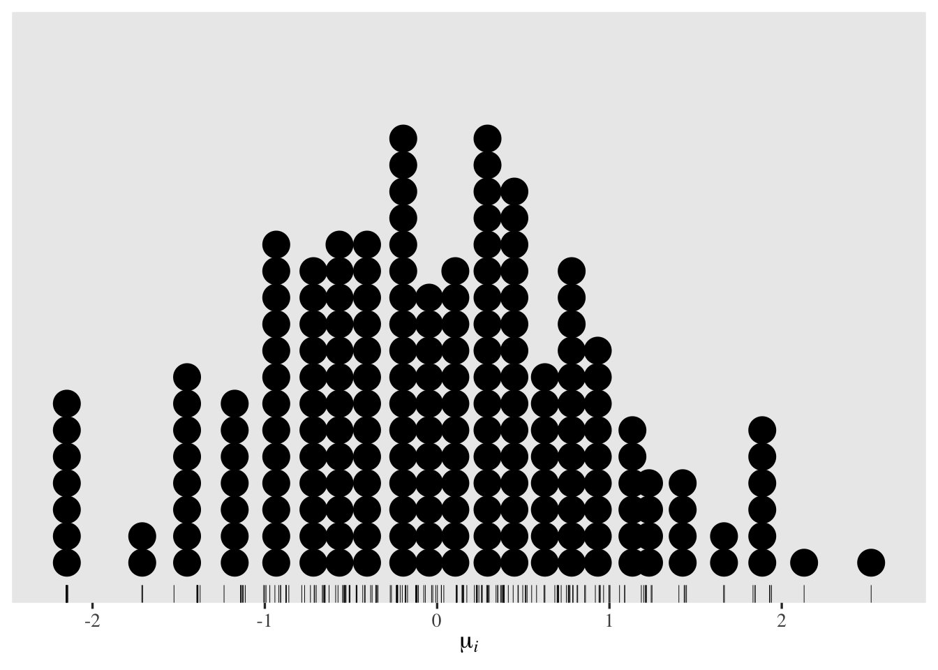
In this case, the \(u_i\) summaries from ranef() will be in the latent-mean metric. This is because the grand mean is still set to \(0\) for identification purposes. Here’s what the posterior means for those parameters look like in a dot plot.

tibble(ranef = ranef(fit4)$id[, 1, "Intercept"]) %>% 
  
  ggplot(aes(x = ranef)) + 
  geom_rug(linewidth = 1/6) +
  geom_dotplot(binwidth = 1/6.5) +
  scale_y_continuous(NULL, breaks = NULL) +
  xlab(expression(mu[italic(i)]))

Now it’s time to fit a proper cross-classified model accounting for the nesting within \(i\) persons and \(j\) questions. That will follow the equation

$$ \begin{align*} p(\text{rating} = k | \{ \tau_k \}, \mu_{i\color{blue}j}) & = \Phi(\tau_k - \mu_{i\color{blue}j}) - \Phi(\tau_{k - 1} - \mu_{i\color{blue}j}) \\ \mu_{i\color{blue}j} & = 0 + u_i \color{blue}{ + } \color{blue}{v_j} \\ u_i & \sim \mathcal N(0, \sigma_u) \\ {\color{blue}{v_j}} & \sim {\color{blue}{\mathcal N(0, \sigma_v)}} \\ \tau_1 & \sim \mathcal N(-0.97, 1) \\ \tau_2 & \sim \mathcal N(-0.43, 1) \\ \tau_3 & \sim \mathcal N(0, 1) \\ \tau_4 & \sim \mathcal N(0.43, 1) \\ \tau_5 & \sim \mathcal N(0.97, 1) \\ \sigma_u & \sim \operatorname{Exponential}(1) \\ {\color{blue}{\sigma_v}} & \sim {\color{blue}{\operatorname{Exponential}(1)}}. \end{align*} $$

At this point, we’re now fitting a Bayesian IRT model along the lines Bürkner showcased in his ( 2020) tutorial. We have person-level parameters in \(u_i\) and item-level parameters in \(v_j\).

Fit the model.

# 1.278795 secs
fit5 <- brm(
  data = d,
  family = cumulative(probit),
  rating ~ 1 + (1 | id) + (1 | item),
  prior = c(prior(normal(-0.97, 1), class = Intercept, coef = 1),
            prior(normal(-0.43, 1), class = Intercept, coef = 2),
            prior(normal( 0.00, 1), class = Intercept, coef = 3),
            prior(normal( 0.43, 1), class = Intercept, coef = 4),
            prior(normal( 0.97, 1), class = Intercept, coef = 5),
            prior(exponential(1), class = sd)),
  cores = 4,
  seed = 1,
  init_r = 0.2
)

Check the summary.

print(fit5)

##  Family: cumulative 
##   Links: mu = probit; disc = identity 
## Formula: rating ~ 1 + (1 | id) + (1 | item) 
##    Data: d (Number of observations: 1000) 
##   Draws: 4 chains, each with iter = 2000; warmup = 1000; thin = 1;
##          total post-warmup draws = 4000
## 
## Group-Level Effects: 
## ~id (Number of levels: 200) 
##               Estimate Est.Error l-95% CI u-95% CI Rhat Bulk_ESS Tail_ESS
## sd(Intercept)     1.04      0.07     0.91     1.19 1.00     1497     2029
## 
## ~item (Number of levels: 5) 
##               Estimate Est.Error l-95% CI u-95% CI Rhat Bulk_ESS Tail_ESS
## sd(Intercept)     0.21      0.12     0.07     0.52 1.00     1455     2003
## 
## Population-Level Effects: 
##              Estimate Est.Error l-95% CI u-95% CI Rhat Bulk_ESS Tail_ESS
## Intercept[1]    -1.36      0.14    -1.64    -1.08 1.00     2167     2333
## Intercept[2]    -0.38      0.13    -0.66    -0.13 1.00     2186     2486
## Intercept[3]     0.08      0.13    -0.19     0.34 1.00     2196     2537
## Intercept[4]     1.04      0.14     0.77     1.31 1.00     2396     2486
## Intercept[5]     1.88      0.15     1.59     2.17 1.00     2731     2506
## 
## Family Specific Parameters: 
##      Estimate Est.Error l-95% CI u-95% CI Rhat Bulk_ESS Tail_ESS
## disc     1.00      0.00     1.00     1.00   NA       NA       NA
## 
## Draws were sampled using sampling(NUTS). For each parameter, Bulk_ESS
## and Tail_ESS are effective sample size measures, and Rhat is the potential
## scale reduction factor on split chains (at convergence, Rhat = 1).

Given there are only five levels of item, we should not be surprised the posterior for \(\sigma_v\) is much more uncertain relative to \(\sigma_u\). It should also not be shocking that the posterior for \(\sigma_v\) is also centered around a relatively small value. These five questions are all from the Neuroticism scale and psychologists tend to publish scales with relatively homogeneous items.

An issue that’s easy to miss with these two models is they’re holding the thresholds constant across both persons and items. At the moment, brms is not capable of hierarchically modeling the thresholds (see this thread), However, one can allow for differnt thresholds by question in a fixed-effects sort of way. Here’s what the updated statistical model would be

$$ \begin{align*} p(\text{rating} = k | \{ \tau_{k\color{blue}j} \}, \mu_{ij}) & = \Phi(\tau_{k\color{blue}j} - \mu_{ij}) - \Phi(\tau_{k - 1,\color{blue}j} - \mu_{ij}) \\ \mu_{ij} & = 0 + u_i + v_j \\ u_i & \sim \mathcal N(0, \sigma_u) \\ v_j & \sim \mathcal N(0, \sigma_v) \\ \tau_{1\color{blue}j} & \sim \mathcal N(-0.97, 1) \\ \tau_{2\color{blue}j} & \sim \mathcal N(-0.43, 1) \\ \tau_{3\color{blue}j} & \sim \mathcal N(0, 1) \\ \tau_{4\color{blue}j} & \sim \mathcal N(0.43, 1) \\ \tau_{5\color{blue}j} & \sim \mathcal N(0.97, 1) \\ \sigma_u & \sim \operatorname{Exponential}(1) \\ \sigma_v & \sim \operatorname{Exponential}(1), \end{align*} $$

where all the \(\tau\) parameters vary across the \(j\) levels of item. To fit such a model with brms, you use the thres(gr = <group>) helper function on the left-hand side of the model formula. If you want to continue to manually set different priors for the thresholds, you’ll now need to include the group argument within the prior() function. In my experience, don’t be surprised if you have to adjust adapt_delta at this point.

# 3.59341 mins
fit6 <- brm(
  data = d,
  family = cumulative(probit),
  rating | thres(gr = item) ~ 1 + (1 | id) + (1 | item),
  prior = c(prior(normal(-0.97, 1), class = Intercept, coef = 1, group = N1),
            prior(normal(-0.43, 1), class = Intercept, coef = 2, group = N1),
            prior(normal( 0.00, 1), class = Intercept, coef = 3, group = N1),
            prior(normal( 0.43, 1), class = Intercept, coef = 4, group = N1),
            prior(normal( 0.97, 1), class = Intercept, coef = 5, group = N1),
            
            prior(normal(-0.97, 1), class = Intercept, coef = 1, group = N2),
            prior(normal(-0.43, 1), class = Intercept, coef = 2, group = N2),
            prior(normal( 0.00, 1), class = Intercept, coef = 3, group = N2),
            prior(normal( 0.43, 1), class = Intercept, coef = 4, group = N2),
            prior(normal( 0.97, 1), class = Intercept, coef = 5, group = N2),
            
            prior(normal(-0.97, 1), class = Intercept, coef = 1, group = N3),
            prior(normal(-0.43, 1), class = Intercept, coef = 2, group = N3),
            prior(normal( 0.00, 1), class = Intercept, coef = 3, group = N3),
            prior(normal( 0.43, 1), class = Intercept, coef = 4, group = N3),
            prior(normal( 0.97, 1), class = Intercept, coef = 5, group = N3),
            
            prior(normal(-0.97, 1), class = Intercept, coef = 1, group = N4),
            prior(normal(-0.43, 1), class = Intercept, coef = 2, group = N4),
            prior(normal( 0.00, 1), class = Intercept, coef = 3, group = N4),
            prior(normal( 0.43, 1), class = Intercept, coef = 4, group = N4),
            prior(normal( 0.97, 1), class = Intercept, coef = 5, group = N4),
            
            prior(normal(-0.97, 1), class = Intercept, coef = 1, group = N5),
            prior(normal(-0.43, 1), class = Intercept, coef = 2, group = N5),
            prior(normal( 0.00, 1), class = Intercept, coef = 3, group = N5),
            prior(normal( 0.43, 1), class = Intercept, coef = 4, group = N5),
            prior(normal( 0.97, 1), class = Intercept, coef = 5, group = N5),
            
            prior(exponential(1), class = sd)),
  cores = 4,
  seed = 1,
  init_r = 0.2,
  control = list(adapt_delta = .99)
)

The summary is now quite lengthy.

print(fit6)

##  Family: cumulative 
##   Links: mu = probit; disc = identity 
## Formula: rating | thres(gr = item) ~ 1 + (1 | id) + (1 | item) 
##    Data: d (Number of observations: 1000) 
##   Draws: 4 chains, each with iter = 2000; warmup = 1000; thin = 1;
##          total post-warmup draws = 4000
## 
## Group-Level Effects: 
## ~id (Number of levels: 200) 
##               Estimate Est.Error l-95% CI u-95% CI Rhat Bulk_ESS Tail_ESS
## sd(Intercept)     1.06      0.08     0.91     1.22 1.01     1416     2119
## 
## ~item (Number of levels: 5) 
##               Estimate Est.Error l-95% CI u-95% CI Rhat Bulk_ESS Tail_ESS
## sd(Intercept)     0.23      0.20     0.01     0.73 1.00     1523     2400
## 
## Population-Level Effects: 
##                 Estimate Est.Error l-95% CI u-95% CI Rhat Bulk_ESS Tail_ESS
## Intercept[N1,1]    -1.30      0.25    -1.87    -0.85 1.00     2717     2195
## Intercept[N1,2]    -0.46      0.24    -1.02    -0.02 1.00     2776     2162
## Intercept[N1,3]    -0.01      0.24    -0.57     0.43 1.00     2809     2281
## Intercept[N1,4]     1.12      0.25     0.56     1.57 1.00     3028     2808
## Intercept[N1,5]     1.99      0.27     1.40     2.47 1.00     3520     2772
## Intercept[N2,1]    -1.80      0.26    -2.33    -1.27 1.00     3003     2569
## Intercept[N2,2]    -0.64      0.24    -1.14    -0.15 1.00     3191     2365
## Intercept[N2,3]    -0.13      0.23    -0.64     0.35 1.00     3103     2017
## Intercept[N2,4]     0.73      0.24     0.24     1.24 1.00     3093     2758
## Intercept[N2,5]     1.75      0.25     1.24     2.28 1.00     3717     3134
## Intercept[N3,1]    -1.43      0.25    -2.02    -0.99 1.00     2855     2498
## Intercept[N3,2]    -0.34      0.24    -0.90     0.10 1.00     2965     2563
## Intercept[N3,3]     0.04      0.24    -0.51     0.48 1.00     3047     2545
## Intercept[N3,4]     1.08      0.25     0.52     1.52 1.00     3096     2459
## Intercept[N3,5]     1.82      0.26     1.23     2.28 1.00     3424     2966
## Intercept[N4,1]    -1.47      0.25    -2.03    -0.99 1.00     2880     2575
## Intercept[N4,2]    -0.58      0.24    -1.15    -0.13 1.00     3112     2709
## Intercept[N4,3]    -0.00      0.24    -0.54     0.45 1.00     3084     2786
## Intercept[N4,4]     0.96      0.24     0.41     1.42 1.00     3264     2669
## Intercept[N4,5]     1.89      0.27     1.32     2.39 1.00     3730     2695
## Intercept[N5,1]    -1.18      0.25    -1.76    -0.74 1.00     2872     2875
## Intercept[N5,2]    -0.23      0.24    -0.80     0.20 1.00     3071     2772
## Intercept[N5,3]     0.22      0.24    -0.34     0.67 1.00     3108     2855
## Intercept[N5,4]     1.04      0.24     0.48     1.48 1.00     3392     3014
## Intercept[N5,5]     1.68      0.26     1.09     2.18 1.00     3633     2985
## 
## Family Specific Parameters: 
##      Estimate Est.Error l-95% CI u-95% CI Rhat Bulk_ESS Tail_ESS
## disc     1.00      0.00     1.00     1.00   NA       NA       NA
## 
## Draws were sampled using sampling(NUTS). For each parameter, Bulk_ESS
## and Tail_ESS are effective sample size measures, and Rhat is the potential
## scale reduction factor on split chains (at convergence, Rhat = 1).

It might be easier to get a sense of the \(\tau_{kj}\) posteriors with a coefficient plot.

posterior_summary(fit6)[1:25, ] %>% 
  data.frame() %>% 
  mutate(tau = rep(1:5, times = 5),
         item = rep(1:5, each = 5)) %>% 
  mutate(tau = str_c("tau[", tau, "]"),
         item = factor(item)) %>% 
  
  ggplot(aes(y = Estimate, ymin = Q2.5, ymax = Q97.5, x = tau,
             group = item, color = item)) +
  geom_pointrange(position = position_dodge(width = -0.5), fatten = 1.5) +
  scale_color_viridis_d(expression(item~(italic(j))), option = "F", end = 0.8, direction = -1) +
  scale_x_discrete(NULL, labels = ggplot2:::parse_safe) +
  coord_flip() +
  ylab(expression(Phi))

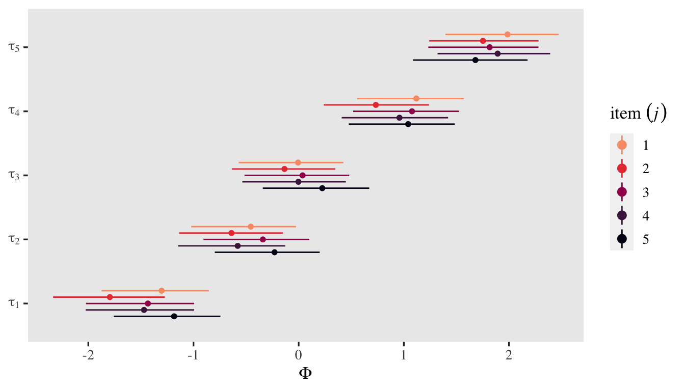
You could use information criteria comparisons to decide on whether to allow them to vary across items or if it’s okay to prefer the more parsimonious model. IMO, thresholds across items are a priori different and should not be collapsed without strong theoretical or methodological justifications. In this case, it seems like I lose nothing by having them.

Plus, there’s also the implications of the varying thresholds for the posterior-predictive distributions.

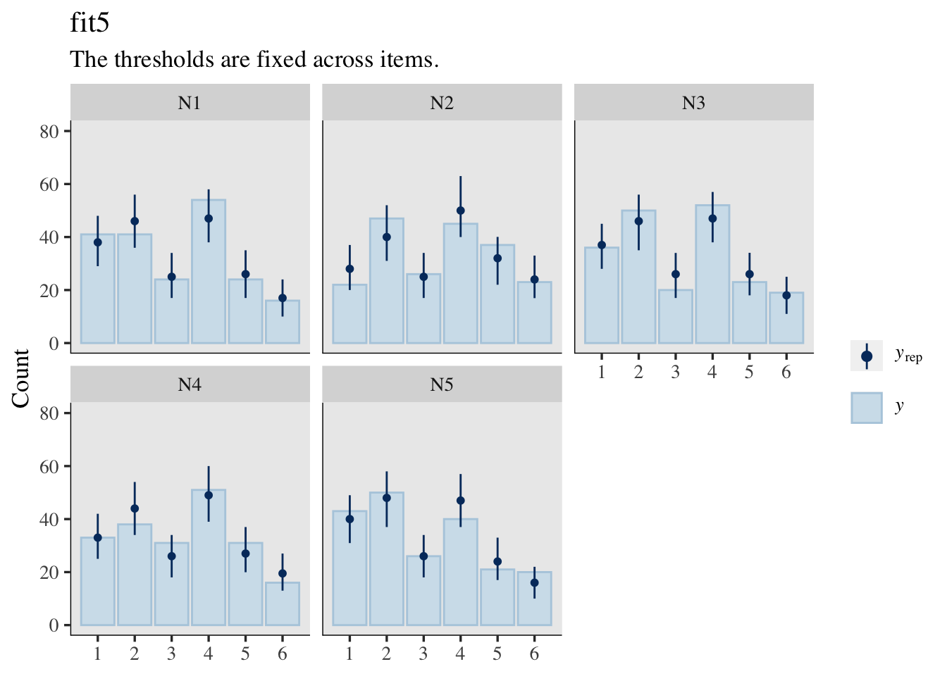
set.seed(1)
pp_check(fit5, type = "bars_grouped", group = "item",
         ndraws = 500, size = 1/2, fatten = 3/2) +
  ylim(0, 80) +
  labs(title = "fit5",
       subtitle = "The thresholds are fixed across items.")

set.seed(1)
pp_check(fit6, type = "bars_grouped", group = "item",
         ndraws = 500, size = 1/2, fatten = 3/2) +
  ylim(0, 80) +
  labs(title = "fit6",
       subtitle = "The thresholds can now vary across items.")

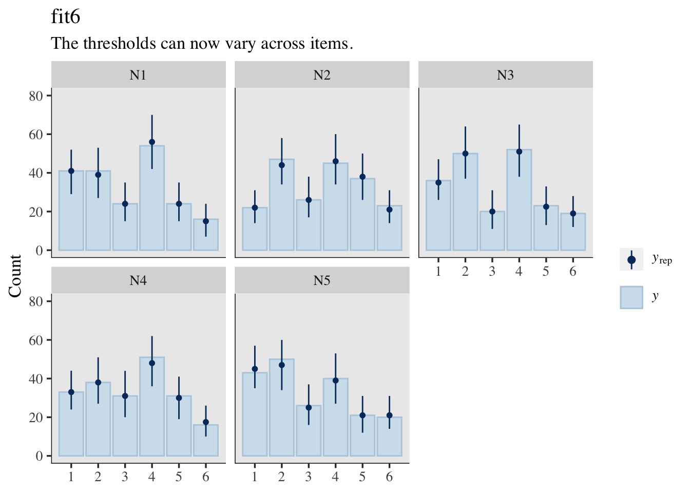
Well okay, maybe I do lose something by letting the thresholds vary across questions. If you look at the parameter summaries for fit5 and fit6, you’ll see the posterior standard deviations (see the Est.Error columns) are wider in fit6. This corresponds to the wider prediction intervals in the pp_check() plot for fit6, compared to the plot for fit5. You might think of this as trade-off of accuracy for precision or of reliability for validity. IMO, the trade-off was worth it. Allowing the thresholds to vary across the items makes for much better posterior predictions.

Randomly-varying latent standard deviations.

If the latent means can vary randomly, the latent dispersion parameters can vary randomly, too. Now \(\log(\alpha_{ij})\) will vary across \(i\) persons and \(j\) questions with the Bayesian ordinal IRT model

$$ \begin{align*} \small{p(\text{rating} = k | \{ \tau_{kj} \}, \mu_{ij}, {\color{blue}{\alpha_{ij}}})} & = \small{\Phi({\color{blue}{\alpha_{ij}}} [\tau_{kj} - \mu_{ij}]) - \Phi( {\color{blue}{\alpha_{ij}}} [\tau_{k - 1,j} - \mu_{ij}])} \\ \mu_{ij} & = 0 + u_i + v_j \\ {\color{blue}{\log(\alpha_{ij})}} & = {\color{blue}{0 + w_i + x_j}} \\ u_i & \sim \mathcal N(0, \sigma_u) \\ v_j & \sim \mathcal N(0, \sigma_v) \\ {\color{blue}{w_i}} & \sim {\color{blue}{\mathcal N(0, \sigma_w)}} \\ {\color{blue}{x_j}} & \sim {\color{blue}{\mathcal N(0, \sigma_x)}} \\ \tau_{1j} & \sim \mathcal N(-0.97, 1) \\ \tau_{2j} & \sim \mathcal N(-0.43, 1) \\ \tau_{3j} & \sim \mathcal N(0, 1) \\ \tau_{4j} & \sim \mathcal N(0.43, 1) \\ \tau_{5j} & \sim \mathcal N(0.97, 1) \\ \sigma_u & \sim \operatorname{Exponential}(1) \\ \sigma_v & \sim \operatorname{Exponential}(1) \\ {\color{blue}{\sigma_w}} & \sim {\color{blue}{\operatorname{Exponential}(1)}} \\ {\color{blue}{\sigma_x}} & \sim {\color{blue}{\operatorname{Exponential}(1)}} . \end{align*} $$

Though the \(\operatorname{Exponential}(1)\) prior might be a good place to start with our new \(\sigma_w\) and \(\sigma_x\), let’s ponder this a bit. Recall these are for the distribution of logged discrimination parameters. Since I’m no statistician or psychometrician, I’m not even sure what that means, which makes it hard to intuit whether the \(\operatorname{Exponential}(1)\) prior makes sense for my data. A plot might help. Here we’ll simulate \(100{,}000\) draws from the \(\operatorname{Exponential}(1)\) prior, use those draws to simulate \(w_i\) values from \(\mathcal N(0, \sigma_w)\), and then plot that distribution in the \(w_i\), \(\exp(w_i)\) and \(1/\exp(w_i)\) metrics.

set.seed(1)

# simulate from the prior
tibble(sigma_w = rexp(n = 1e5, rate = 1)) %>% 
  # simulate w_i draws
  mutate(`italic(w[i])` = rnorm(n = n(), mean = 0, sd = sigma_w)) %>% 
  # transform
  mutate(`exp(italic(w[i]))` = exp(`italic(w[i])`)) %>% 
  mutate(`1/exp(italic(w[i]))` = 1 / `exp(italic(w[i]))`) %>% 
  # wrangle
  pivot_longer(-sigma_w) %>% 
  mutate(name = factor(name, levels = c("italic(w[i])", "exp(italic(w[i]))", "1/exp(italic(w[i]))"))) %>% 
  # for computational simplicity, remove some values from the far right tail
  filter(value < 100) %>% 
  
  # plot!
  ggplot(aes(x = value)) +
  geom_histogram(binwidth = 0.1) +
  scale_y_continuous(NULL, breaks = NULL) +
  coord_cartesian(xlim = c(-10, 10)) +
  ggtitle(expression("Prior predictive distribution for "*sigma[italic(w)]%~%Exponential(1))) +
  facet_wrap(~ name, labeller = label_parsed, ncol = 1)

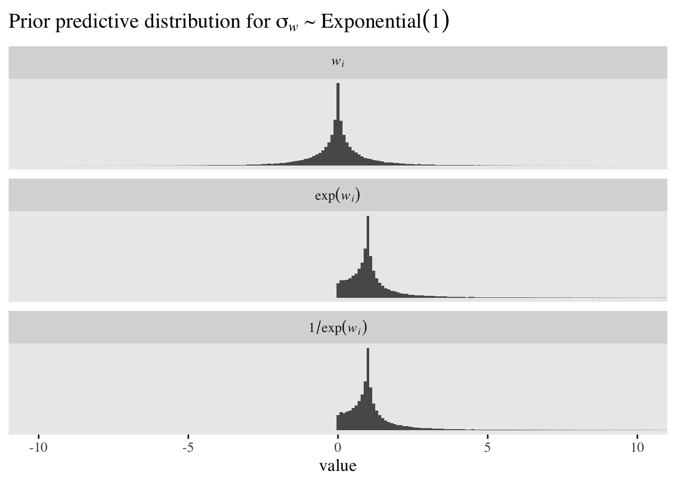
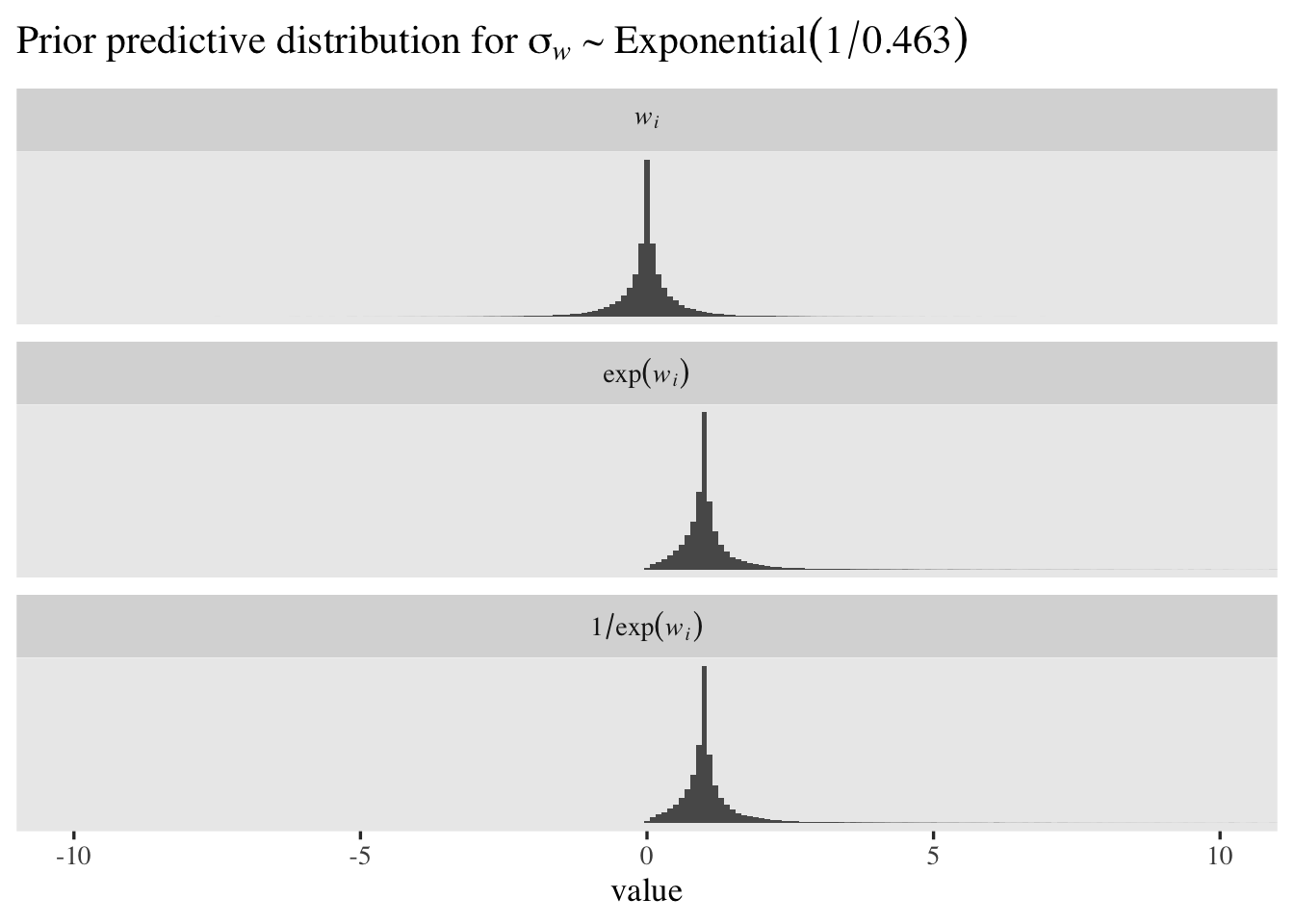
The mean and median for \(w_i\) are both zero. Because of the very long right tails, both \(\exp(w_i)\) and \(1/\exp(w_i)\) have very large means and standard deviations. However, both \(\exp(w_i)\) and \(1/\exp(w_i)\) have medians at \(1\). The \(1/\exp(w_i)\) distribution is the one that’s in the latent \(\sigma\) metric and its percentile-based 95% interval ranges from \(0.05\) to \(20.28\). That isn’t bad for a permissive level-2 standard deviation prior, but I think we can do better. If we set the mean of the exponential prior to \(0.463\), the resulting prior-predictive distribution of \(1/\exp(w_i)\) will have a percentile-based 95% interval of \(0.25\) to \(4\). Here’s what that looks like.

set.seed(1)

# save for this first line, this workflow is the same as before
tibble(sigma_w = rexp(n = 1e5, rate = 1 / 0.463)) %>% 
  mutate(`italic(w[i])` = rnorm(n = n(), mean = 0, sd = sigma_w)) %>% 
  mutate(`exp(italic(w[i]))` = exp(`italic(w[i])`)) %>% 
  mutate(`1/exp(italic(w[i]))` = 1 / `exp(italic(w[i]))`) %>% 
  pivot_longer(-sigma_w) %>% 
  mutate(name = factor(name, levels = c("italic(w[i])", "exp(italic(w[i]))", "1/exp(italic(w[i]))"))) %>% 
  filter(value < 100) %>% 
  
  ggplot(aes(x = value)) +
  geom_histogram(binwidth = 0.1) +
  scale_y_continuous(NULL, breaks = NULL) +
  coord_cartesian(xlim = c(-10, 10)) +
  ggtitle(expression("Prior predictive distribution for "*sigma[italic(w)]%~%Exponential(1/0.463))) +
  facet_wrap(~ name, labeller = label_parsed, ncol = 1)

With that as our prior, our updated model formula will be

$$ \begin{align*} \small{p(\text{rating} = k | \{ \tau_{kj} \}, \mu_{ij}, \alpha_{ij})} & = \small{\Phi(\alpha_{ij}[\tau_{kj} - \mu_{ij}]) - \Phi(\alpha_{ij}[\tau_{k - 1,j} - \mu_{ij}])} \\ \mu_{ij} & = 0 + u_i + v_j \\ \log(\alpha_{ij}) & = 0 + w_i + x_j \\ u_i & \sim \mathcal N(0, \sigma_u) \\ v_j & \sim \mathcal N(0, \sigma_v) \\ w_i & \sim \mathcal N(0, \sigma_w) \\ x_j & \sim \mathcal N(0, \sigma_x) \\ \tau_{1j} & \sim \mathcal N(-0.97, 1) \\ \tau_{2j} & \sim \mathcal N(-0.43, 1) \\ \tau_{3j} & \sim \mathcal N(0, 1) \\ \tau_{4j} & \sim \mathcal N(0.43, 1) \\ \tau_{5j} & \sim \mathcal N(0.97, 1) \\ \sigma_u & \sim \operatorname{Exponential}(1) \\ \sigma_v & \sim \operatorname{Exponential}(1) \\ \sigma_w & \sim \operatorname{Exponential}({\color{blue}{1 / 0.463}} ) \\ \sigma_x & \sim \operatorname{Exponential}({\color{blue}{1 / 0.463}} ). \end{align*} $$

Put those new priors to work and fit the model.

# 5.223564 mins
fit7 <- brm(
  data = d,
  family = cumulative(probit),
  bf(rating | thres(gr = item) ~ 1 + (1 | id) + (1 | item)) +
    lf(disc ~ 0 + (1 | id) + (1 | item)),
  prior = c(prior(normal(-0.97, 1), class = Intercept, coef = 1, group = N1),
            prior(normal(-0.43, 1), class = Intercept, coef = 2, group = N1),
            prior(normal( 0.00, 1), class = Intercept, coef = 3, group = N1),
            prior(normal( 0.43, 1), class = Intercept, coef = 4, group = N1),
            prior(normal( 0.97, 1), class = Intercept, coef = 5, group = N1),
            
            prior(normal(-0.97, 1), class = Intercept, coef = 1, group = N2),
            prior(normal(-0.43, 1), class = Intercept, coef = 2, group = N2),
            prior(normal( 0.00, 1), class = Intercept, coef = 3, group = N2),
            prior(normal( 0.43, 1), class = Intercept, coef = 4, group = N2),
            prior(normal( 0.97, 1), class = Intercept, coef = 5, group = N2),
            
            prior(normal(-0.97, 1), class = Intercept, coef = 1, group = N3),
            prior(normal(-0.43, 1), class = Intercept, coef = 2, group = N3),
            prior(normal( 0.00, 1), class = Intercept, coef = 3, group = N3),
            prior(normal( 0.43, 1), class = Intercept, coef = 4, group = N3),
            prior(normal( 0.97, 1), class = Intercept, coef = 5, group = N3),
            
            prior(normal(-0.97, 1), class = Intercept, coef = 1, group = N4),
            prior(normal(-0.43, 1), class = Intercept, coef = 2, group = N4),
            prior(normal( 0.00, 1), class = Intercept, coef = 3, group = N4),
            prior(normal( 0.43, 1), class = Intercept, coef = 4, group = N4),
            prior(normal( 0.97, 1), class = Intercept, coef = 5, group = N4),
            
            prior(normal(-0.97, 1), class = Intercept, coef = 1, group = N5),
            prior(normal(-0.43, 1), class = Intercept, coef = 2, group = N5),
            prior(normal( 0.00, 1), class = Intercept, coef = 3, group = N5),
            prior(normal( 0.43, 1), class = Intercept, coef = 4, group = N5),
            prior(normal( 0.97, 1), class = Intercept, coef = 5, group = N5),
            
            prior(exponential(1), class = sd),
            # here's the fancy new prior line
            prior(exponential(1 / 0.463), class = sd, dpar = disc)),
  cores = 4,
  seed = 1,
  init_r = 0.2,
  control = list(adapt_delta = .99)
)

Summarize.

print(fit7)

##  Family: cumulative 
##   Links: mu = probit; disc = log 
## Formula: rating | thres(gr = item) ~ 1 + (1 | id) + (1 | item) 
##          disc ~ 0 + (1 | id) + (1 | item)
##    Data: d (Number of observations: 1000) 
##   Draws: 4 chains, each with iter = 2000; warmup = 1000; thin = 1;
##          total post-warmup draws = 4000
## 
## Group-Level Effects: 
## ~id (Number of levels: 200) 
##                    Estimate Est.Error l-95% CI u-95% CI Rhat Bulk_ESS Tail_ESS
## sd(Intercept)          1.19      0.14     0.92     1.49 1.00      567     1045
## sd(disc_Intercept)     0.44      0.06     0.34     0.56 1.00     1322     2459
## 
## ~item (Number of levels: 5) 
##                    Estimate Est.Error l-95% CI u-95% CI Rhat Bulk_ESS Tail_ESS
## sd(Intercept)          0.26      0.23     0.01     0.85 1.00     1451     1997
## sd(disc_Intercept)     0.42      0.18     0.17     0.87 1.00     1101     1271
## 
## Population-Level Effects: 
##                 Estimate Est.Error l-95% CI u-95% CI Rhat Bulk_ESS Tail_ESS
## Intercept[N1,1]    -1.32      0.30    -1.99    -0.77 1.00     1191     2072
## Intercept[N1,2]    -0.50      0.26    -1.09    -0.02 1.00     2149     2864
## Intercept[N1,3]    -0.06      0.25    -0.65     0.41 1.00     2637     2862
## Intercept[N1,4]     1.04      0.28     0.40     1.56 1.00     1859     3117
## Intercept[N1,5]     1.91      0.35     1.21     2.60 1.00     1311     2212
## Intercept[N2,1]    -1.81      0.33    -2.47    -1.17 1.00     1012     2135
## Intercept[N2,2]    -0.60      0.25    -1.08    -0.09 1.00     2020     2854
## Intercept[N2,3]    -0.12      0.24    -0.58     0.40 1.00     2941     2942
## Intercept[N2,4]     0.69      0.25     0.21     1.21 1.00     2323     2732
## Intercept[N2,5]     1.67      0.32     1.07     2.34 1.00     1441     2250
## Intercept[N3,1]    -1.52      0.33    -2.28    -0.96 1.00      980     1378
## Intercept[N3,2]    -0.36      0.27    -0.98     0.11 1.00     1980     2461
## Intercept[N3,3]     0.03      0.26    -0.56     0.51 1.00     2597     2703
## Intercept[N3,4]     1.18      0.29     0.55     1.74 1.00     2283     2869
## Intercept[N3,5]     2.08      0.37     1.36     2.83 1.00     1519     2576
## Intercept[N4,1]    -1.89      0.36    -2.63    -1.24 1.00     1058     2321
## Intercept[N4,2]    -0.73      0.28    -1.35    -0.23 1.00     2103     2903
## Intercept[N4,3]    -0.02      0.26    -0.59     0.47 1.00     3276     3331
## Intercept[N4,4]     1.21      0.30     0.58     1.81 1.00     2084     2892
## Intercept[N4,5]     2.57      0.44     1.74     3.50 1.00     1276     2514
## Intercept[N5,1]    -1.66      0.37    -2.53    -1.07 1.00     1009     1687
## Intercept[N5,2]    -0.35      0.29    -1.04     0.13 1.00     2181     2105
## Intercept[N5,3]     0.25      0.29    -0.42     0.74 1.00     2767     2573
## Intercept[N5,4]     1.40      0.34     0.68     2.04 1.00     2143     2835
## Intercept[N5,5]     2.40      0.42     1.58     3.25 1.00     1596     2798
## 
## Draws were sampled using sampling(NUTS). For each parameter, Bulk_ESS
## and Tail_ESS are effective sample size measures, and Rhat is the potential
## scale reduction factor on split chains (at convergence, Rhat = 1).

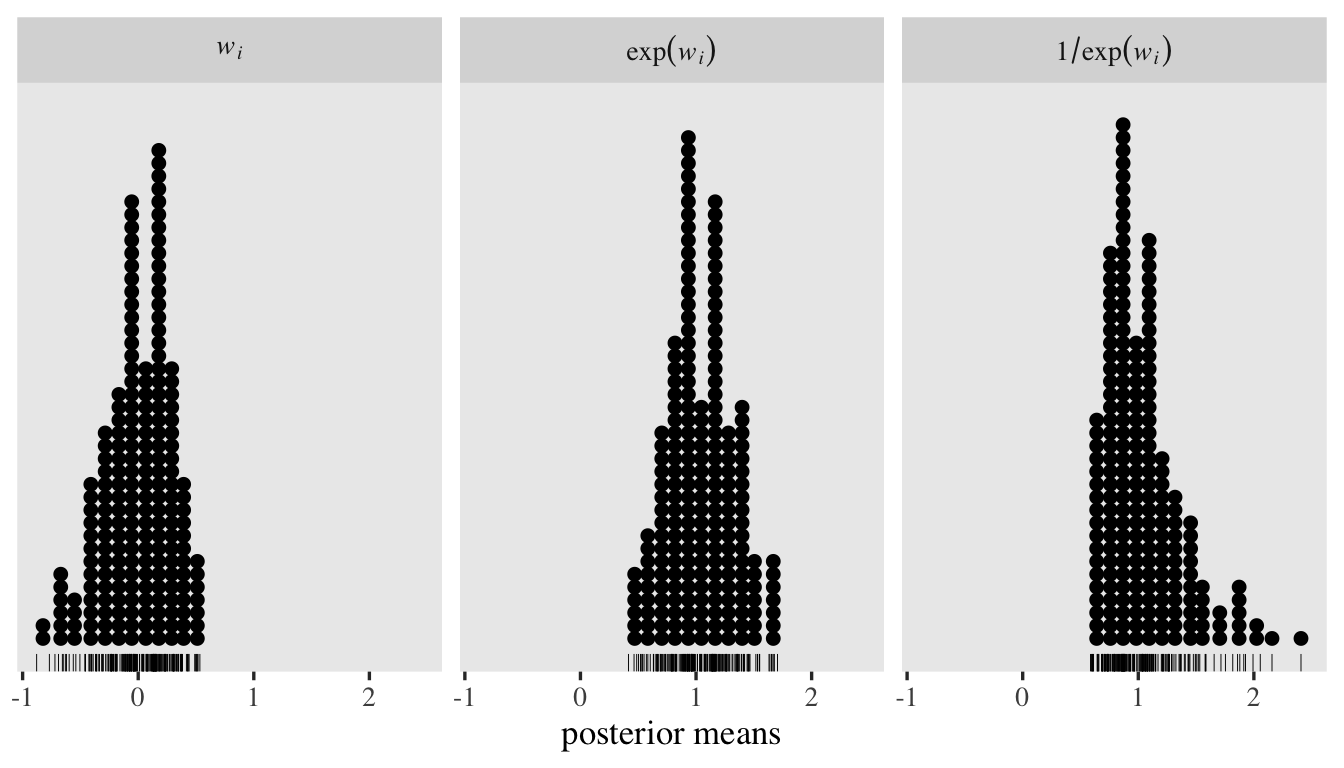
To get a better sense of what those new level-2 random \(\log(\alpha_{ij})\) standard deviation estimates mean, let’s focus on the posterior for \(\sigma_w\), which is \(0.44, 95\% \text{CI}\ [0.34, 0.56]\). We can use the ranef() function to pull the summary statistics for the corresponding \(w_i\) posteriors. To simplify things, we’ll just focus on the posterior means. After pulling the summaries, we’ll place them within a tibble, transform them to the \(\exp(w_i)\) and \(1 / \exp(w_i)\) metrics, and then plot like with the prior predictive distributions, before. But since we only have \(200\) values to visualize, this time, we’ll use dot plots.

tibble(`italic(w[i])` = ranef(fit7)$id[, 1, "disc_Intercept"]) %>% 
  mutate(`exp(italic(w[i]))` = exp(`italic(w[i])`)) %>% 
  mutate(`1/exp(italic(w[i]))` = 1 / exp(`italic(w[i])`)) %>% 
  pivot_longer(everything()) %>% 
  mutate(name = factor(name, levels = c("italic(w[i])", "exp(italic(w[i]))", "1/exp(italic(w[i]))"))) %>% 
  
  ggplot(aes(x = value)) + 
  geom_rug(linewidth = 1/6) +
  geom_dotplot(binwidth = 1/9) +
  scale_y_continuous(NULL, breaks = NULL) +
  xlab("posterior means") +
  facet_wrap(~ name, labeller = label_parsed)

Now we turn to the task of using the model to compute the means of the rating variable, this time separately for each of the \(5\) Neuroticism items. One could generalized the workflow we used for fit1 through fit3, but I wouldn’t recommend that. The brms::fitted() function will be our friend, here. Though ultimately we’ll want to use fitted() with summary = FALSE, I’m going to save the results both ways to help explain the output.

# define the new data
nd <- d %>% distinct(item)

# save the summarized results
f_summary <-
  fitted(fit7,
         newdata = nd,
         # note this line
         re_formula = ~ (1 | item))

# save the un-summarized results
f <-
  fitted(fit7,
         newdata = nd,
         re_formula = ~ (1 | item),
         summary = F)

First take a look at the structure of f_summary.

f_summary %>% str()

##  num [1:5, 1:4, 1:6] 0.0423 0.0055 0.0852 0.0998 0.1538 ...
##  - attr(*, "dimnames")=List of 3
##   ..$ : NULL
##   ..$ : chr [1:4] "Estimate" "Est.Error" "Q2.5" "Q97.5"
##   ..$ : chr [1:6] "P(Y = 1)" "P(Y = 2)" "P(Y = 3)" "P(Y = 4)" ...

We have a \(3\)-dimensional array. The \(5\) levels of the first dimension are the \(5\) levels of item. The \(4\) levels of the second dimension are the typical summary statistics, the posterior mean through the upper-level of the 95% CI. The \(6\) levels of the third dimension let us divide up the results by the \(6\) levels of \(k\), the rating levels 1 through 6.

But we don’t want summarized results. We want the posterior draws. Enter f.

f %>% str()

##  num [1:4000, 1:5, 1:6] 0.0644 0.049 0.0359 0.0493 0.0258 ...
##  - attr(*, "dimnames")=List of 3
##   ..$ : chr [1:4000] "1" "2" "3" "4" ...
##   ..$ : NULL
##   ..$ : chr [1:6] "1" "2" "3" "4" ...

Now the dimension within the array is the \(4{,}000\) posterior draws. The second dimension is our \(5\) levels of item and the third dimension the \(6\) levels of \(k\). Before we put this all to use, we’ll want to save a few values as external objects for the plotting.

# sample means for the items
m_n1 <- d %>% filter(item == "N1") %>% summarise(m = mean(rating)) %>% pull()
m_n2 <- d %>% filter(item == "N2") %>% summarise(m = mean(rating)) %>% pull()
m_n3 <- d %>% filter(item == "N3") %>% summarise(m = mean(rating)) %>% pull()
m_n4 <- d %>% filter(item == "N4") %>% summarise(m = mean(rating)) %>% pull()
m_n5 <- d %>% filter(item == "N5") %>% summarise(m = mean(rating)) %>% pull()

# save color values for the geom_vline() lines
colors <- viridis::viridis_pal(option = "A", end = 0.85, direction = -1)(5)

Okay, within rbind(), we serially stack the levels of the third dimension within the f array so we can use our tidyverse-style wrangling. Then the workflow looks a lot like before.

rbind(f[, , 1],
      f[, , 2],
      f[, , 3],
      f[, , 4],
      f[, , 5],
      f[, , 6]) %>% 
  data.frame() %>% 
  set_names(str_c("N", 1:5)) %>% 
  mutate(draw   = rep(1:4000, times = 6),
         rating = rep(1:6, each = 4000)) %>% 
  pivot_longer(N1:N5, names_to = "item", values_to = "p") %>% 
  mutate(`p * k` = p * rating) %>% 
  group_by(draw, item) %>% 
  summarise(mean_rating = sum(`p * k`)) %>% 
  
  ggplot(aes(x = mean_rating, y = fct_rev(item), fill = item)) +
  stat_halfeye(.width = .95) +
  geom_vline(xintercept = m_n1, linetype = 2, color = colors[1]) +
  geom_vline(xintercept = m_n2, linetype = 2, color = colors[2]) +
  geom_vline(xintercept = m_n3, linetype = 2, color = colors[3]) +
  geom_vline(xintercept = m_n4, linetype = 2, color = colors[4]) +
  geom_vline(xintercept = m_n5, linetype = 2, color = colors[5]) +
  scale_fill_viridis_d(NULL, option = "A", end = 0.85, direction = -1, alpha = 2/3) +
  labs(title = "The postrior for the mean of the rating values, by item",
       subtitle = "The dashed vertical lines mark off the sample means, by item. The posterior distributions\nare based on the multilevel unconditional distributional cumulative ordinal model fit7.",
       x = expression(mu[rating]),
       y = NULL) +
  xlim(2, 4)

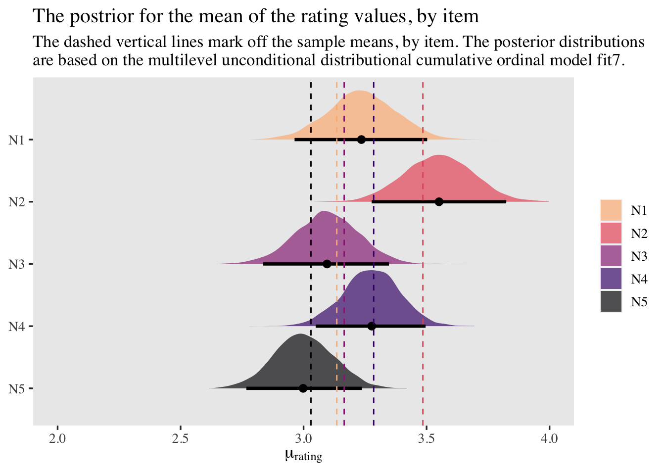
At first glance, it might be upsetting that out posteriors for the item-level means no longer tightly line up with the sample means. However, keep in mind these were computed with a multilevel model, which will impose partial pooling toward the grand mean. Based on decades of hard work within statistics (see Efron & Morris, 1977), we know that our partially-pooled means will be more likely generalize to new data than our sample means. This is why we model. Though we do want to understand our sample data, we also want to make inferences about other data from the population.

Now that we have a full model accounting for all five Neuroticism items, we can use a similar approach to compute the population-level sum score. First, we’ll compute the sample mean of the sum score and save the value as m_sum_score.

m_sum_score <- d %>% 
  group_by(id) %>% 
  summarise(sum = sum(rating)) %>% 
  summarise(mean_sum = mean(sum)) %>% 
  pull()

# what's the value?
m_sum_score

## [1] 16.1

Next we make a small amendment the workflow above. Instead of grouping by posterior draw and by item before the summarise() line, this time we only group by draw. As a consequence, the values for all the items will be summed within each posterior draw, making a vector of sum scores. Then we plot.

rbind(f[, , 1],
      f[, , 2],
      f[, , 3],
      f[, , 4],
      f[, , 5],
      f[, , 6]) %>% 
  data.frame() %>% 
  set_names(str_c("N", 1:5)) %>% 
  mutate(draw   = rep(1:4000, times = 6),
         rating = rep(1:6, each = 4000)) %>% 
  pivot_longer(N1:N5, names_to = "item", values_to = "p") %>% 
  mutate(`p * k` = p * rating) %>% 
  # notice we are no longer grouping by draw AND item
  group_by(draw) %>% 
  summarise(mean_sum_score = sum(`p * k`)) %>% 
  
  ggplot(aes(x = mean_sum_score, y = 0)) +
  stat_halfeye(.width = .95) +
  geom_vline(xintercept = m_sum_score, linetype = 2) +
  scale_y_continuous(NULL, breaks = NULL) +
  labs(title = "The postrior for the mean of the Neuroticism sum cores",
       subtitle = "The dashed vertical lines mark off the sample means. The posterior distributions are based on\nthe multilevel unconditional distributional cumulative ordinal model fit7.",
       x = expression(mu[Neuroticism~sum~score]),
       y = NULL) +
  xlim(10, 20)

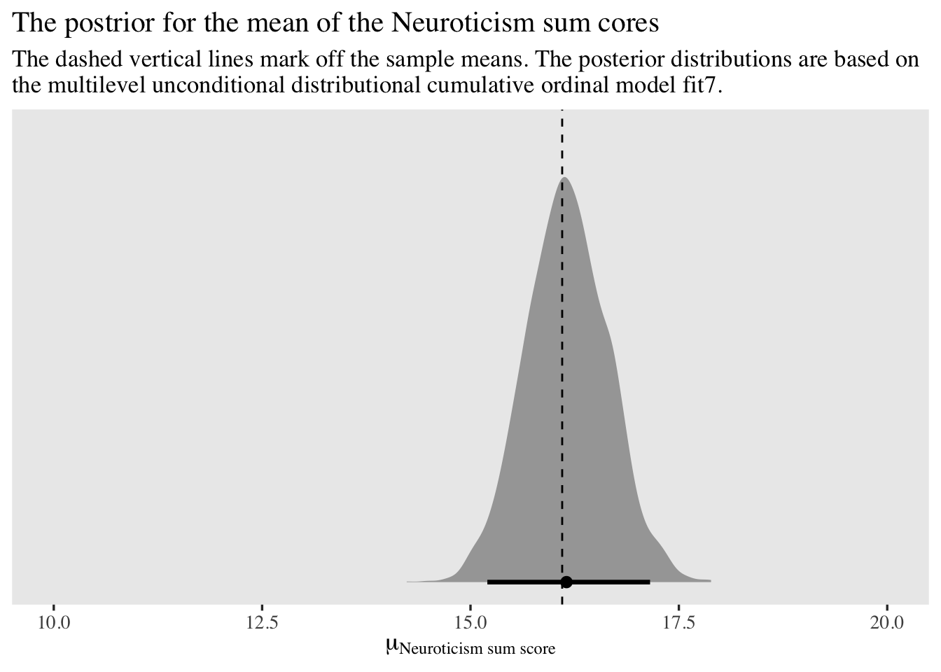
The model does a great job capturing the Neuroticism sum scores.

Now if you wanted to, you could expand this model further to include correlations between \(u_i\) and \(w_i\) and between \(v_j\) and \(x_j\). That would change the model formula to something like

$$ \begin{align*} \small{p(\text{rating} = k | \{ \tau_{kj} \}, \mu_{ij}, \alpha_{ij})} & = \small{\Phi(\alpha_{ij}[\tau_{kj} - \mu_{ij}]) - \Phi(\alpha_{ij}[\tau_{k - 1,j} - \mu_{ij}])} \\ \mu_{ij} & = 0 + u_i + v_j \\ \log(\alpha_{ij}) & = 0 + w_i + x_j \\ \begin{bmatrix} u_i \\ w_i \end{bmatrix} & \sim \mathcal{MVN}(\mathbf 0, \mathbf{S_a {\color{blue}{R_a}} S_a}) \\ \begin{bmatrix} v_j \\ x_j \end{bmatrix} & \sim \mathcal{MVN}(\mathbf 0, \mathbf{S_b {\color{blue}{R_b}} S_b}) \\ \mathbf{S_a} & = \begin{bmatrix} \sigma_u & 0 \\ 0 & \sigma_w \end{bmatrix} \\ \mathbf{S_b} & = \begin{bmatrix} \sigma_v & 0 \\ 0 & \sigma_x \end{bmatrix} \\ {\color{blue}{\mathbf{R_a}}} & = {\color{blue}{\begin{bmatrix} 1 & \rho_a \\ \rho_a & 1 \end{bmatrix}}} \\ {\color{blue}{\mathbf{R_b}}} & = {\color{blue}{\begin{bmatrix} 1 & \rho_b \\ \rho_b & 1 \end{bmatrix}}} \\ \tau_{1j} & \sim \mathcal N(-0.97, 1) \\ \tau_{2j} & \sim \mathcal N(-0.43, 1) \\ \tau_{3j} & \sim \mathcal N(0, 1) \\ \tau_{4j} & \sim \mathcal N(0.43, 1) \\ \tau_{5j} & \sim \mathcal N(0.97, 1) \\ \sigma_u & \sim \operatorname{Exponential}(1) \\ \sigma_v & \sim \operatorname{Exponential}(1) \\ \sigma_w & \sim \operatorname{Exponential}(1 / 0.463) \\ \sigma_x & \sim \operatorname{Exponential}(1 / 0.463) \\ {\color{blue}{\rho_a}} & \sim {\color{blue}{\operatorname{LKJ}(2)}} \\ {\color{blue}{\rho_b}} & \sim {\color{blue}{\operatorname{LKJ}(2)}}, \end{align*} $$

where though our four random parameters are now modeled as two bivariate-normal pairs, there really are only two new parameters: \(\rho_a\) and \(\rho_b\). The LKJ priors for our two new parameters would be weakly regularizing. In my experience, so far, adding those two level-2 correlations can make for notably longer fitting times and they often result in computational complications like the need to further adjust adapt_delta and so on. So in the interest of space, I’m not going to fit this model. But it’s always a possibility to consider.

Full conditional distributional model.

A while back, we put our level-1 predictor male to the side while we focused on expanding the random components. Now’s time to bring that predictor back and fit the full conditional distributional model

$$ \begin{align*} \small{p(\text{rating} = k | \{ \tau_{kj} \}, \mu_{ij}, \alpha_{ij})} & = \small{\Phi(\alpha_{ij}[\tau_{kj} - \mu_{ij}]) - \Phi(\alpha_{ij}[\tau_{k - 1,j} - \mu_{ij}])} \\ \mu_{ij} & = {\color{blue}{\beta_1 \text{male}_i}} + u_i + v_j \\ \log(\alpha_{ij}) & = {\color{blue}{\eta_1 \text{male}_i}} + w_i + x_j \\ u_i & \sim \mathcal N(0, \sigma_u) \\ v_j & \sim \mathcal N(0, \sigma_v) \\ w_i & \sim \mathcal N(0, \sigma_w) \\ x_j & \sim \mathcal N(0, \sigma_x) \\ \tau_{1j} & \sim \mathcal N(-0.97, 1) \\ \tau_{2j} & \sim \mathcal N(-0.43, 1) \\ \tau_{3j} & \sim \mathcal N(0, 1) \\ \tau_{4j} & \sim \mathcal N(0.43, 1) \\ \tau_{5j} & \sim \mathcal N(0.97, 1) \\ {\color{blue}{\beta_1}} & \sim {\color{blue}{\mathcal N(0, 1)}} \\ {\color{blue}{\eta_1}} & \sim {\color{blue}{\mathcal N(0, 0.347)}} \\ \sigma_u & \sim \operatorname{Exponential}(1) \\ \sigma_v & \sim \operatorname{Exponential}(1) \\ \sigma_w & \sim \operatorname{Exponential}(1 / 0.463) \\ \sigma_x & \sim \operatorname{Exponential}(1 / 0.463). \end{align*} $$

At this point, the change to the brms code is trivial.

# 5.223564 mins
fit8 <- brm(
  data = d,
  family = cumulative(probit),
  bf(rating | thres(gr = item) ~ 1 + male + (1 | id) + (1 | item)) +
    lf(disc                    ~ 0 + male + (1 | id) + (1 | item),
       # don't forget this line
       cmc = FALSE),
  prior = c(prior(normal(-0.97, 1), class = Intercept, coef = 1, group = N1),
            prior(normal(-0.43, 1), class = Intercept, coef = 2, group = N1),
            prior(normal( 0.00, 1), class = Intercept, coef = 3, group = N1),
            prior(normal( 0.43, 1), class = Intercept, coef = 4, group = N1),
            prior(normal( 0.97, 1), class = Intercept, coef = 5, group = N1),
            
            prior(normal(-0.97, 1), class = Intercept, coef = 1, group = N2),
            prior(normal(-0.43, 1), class = Intercept, coef = 2, group = N2),
            prior(normal( 0.00, 1), class = Intercept, coef = 3, group = N2),
            prior(normal( 0.43, 1), class = Intercept, coef = 4, group = N2),
            prior(normal( 0.97, 1), class = Intercept, coef = 5, group = N2),
            
            prior(normal(-0.97, 1), class = Intercept, coef = 1, group = N3),
            prior(normal(-0.43, 1), class = Intercept, coef = 2, group = N3),
            prior(normal( 0.00, 1), class = Intercept, coef = 3, group = N3),
            prior(normal( 0.43, 1), class = Intercept, coef = 4, group = N3),
            prior(normal( 0.97, 1), class = Intercept, coef = 5, group = N3),
            
            prior(normal(-0.97, 1), class = Intercept, coef = 1, group = N4),
            prior(normal(-0.43, 1), class = Intercept, coef = 2, group = N4),
            prior(normal( 0.00, 1), class = Intercept, coef = 3, group = N4),
            prior(normal( 0.43, 1), class = Intercept, coef = 4, group = N4),
            prior(normal( 0.97, 1), class = Intercept, coef = 5, group = N4),
            
            prior(normal(-0.97, 1), class = Intercept, coef = 1, group = N5),
            prior(normal(-0.43, 1), class = Intercept, coef = 2, group = N5),
            prior(normal( 0.00, 1), class = Intercept, coef = 3, group = N5),
            prior(normal( 0.43, 1), class = Intercept, coef = 4, group = N5),
            prior(normal( 0.97, 1), class = Intercept, coef = 5, group = N5),
            
            # add those beta and eta priors back in
            prior(normal(0, 1), class = b),
            prior(normal(0, log(2) / 2), class = b, dpar = disc),
            
            prior(exponential(1), class = sd),
            prior(exponential(1 / 0.463), class = sd, dpar = disc)),
  cores = 4,
  seed = 1,
  init_r = 0.2,
  control = list(adapt_delta = .99)
)

Check one last model summary.

print(fit8)

##  Family: cumulative 
##   Links: mu = probit; disc = log 
## Formula: rating | thres(gr = item) ~ 1 + male + (1 | id) + (1 | item) 
##          disc ~ 0 + male + (1 | id) + (1 | item)
##    Data: d (Number of observations: 1000) 
##   Draws: 4 chains, each with iter = 2000; warmup = 1000; thin = 1;
##          total post-warmup draws = 4000
## 
## Group-Level Effects: 
## ~id (Number of levels: 200) 
##                    Estimate Est.Error l-95% CI u-95% CI Rhat Bulk_ESS Tail_ESS
## sd(Intercept)          1.19      0.14     0.95     1.48 1.01      561     1269
## sd(disc_Intercept)     0.45      0.06     0.34     0.57 1.00     1176     2156
## 
## ~item (Number of levels: 5) 
##                    Estimate Est.Error l-95% CI u-95% CI Rhat Bulk_ESS Tail_ESS
## sd(Intercept)          0.23      0.22     0.01     0.80 1.00     1568     2267
## sd(disc_Intercept)     0.39      0.18     0.13     0.83 1.01      692     1015
## 
## Population-Level Effects: 
##                 Estimate Est.Error l-95% CI u-95% CI Rhat Bulk_ESS Tail_ESS
## Intercept[N1,1]    -1.41      0.28    -2.02    -0.88 1.01     1083     1934
## Intercept[N1,2]    -0.57      0.24    -1.10    -0.11 1.00     1649     2840
## Intercept[N1,3]    -0.13      0.23    -0.62     0.31 1.00     2094     2754
## Intercept[N1,4]     0.99      0.26     0.44     1.49 1.00     1695     2870
## Intercept[N1,5]     1.88      0.33     1.26     2.55 1.00     1190     2227
## Intercept[N2,1]    -1.91      0.34    -2.57    -1.25 1.00      903     1806
## Intercept[N2,2]    -0.68      0.25    -1.18    -0.14 1.00     1448     2595
## Intercept[N2,3]    -0.19      0.24    -0.66     0.34 1.00     2032     2858
## Intercept[N2,4]     0.63      0.24     0.17     1.18 1.00     2180     2880
## Intercept[N2,5]     1.62      0.30     1.07     2.26 1.00     1541     2157
## Intercept[N3,1]    -1.56      0.31    -2.23    -0.99 1.01      969     1801
## Intercept[N3,2]    -0.41      0.25    -0.97     0.05 1.00     1992     2320
## Intercept[N3,3]    -0.02      0.25    -0.57     0.43 1.00     2405     2756
## Intercept[N3,4]     1.12      0.28     0.52     1.65 1.00     2068     2839
## Intercept[N3,5]     2.02      0.35     1.35     2.71 1.00     1515     2714
## Intercept[N4,1]    -1.93      0.34    -2.67    -1.30 1.01      930     1596
## Intercept[N4,2]    -0.79      0.26    -1.38    -0.30 1.00     1480     2240
## Intercept[N4,3]    -0.08      0.25    -0.64     0.40 1.00     2758     2591
## Intercept[N4,4]     1.13      0.29     0.54     1.71 1.00     1781     2485
## Intercept[N4,5]     2.48      0.42     1.68     3.35 1.00     1169     1994
## Intercept[N5,1]    -1.66      0.33    -2.39    -1.06 1.01      985     1521
## Intercept[N5,2]    -0.38      0.27    -0.99     0.09 1.00     1916     2387
## Intercept[N5,3]     0.20      0.26    -0.36     0.68 1.00     2610     2768
## Intercept[N5,4]     1.33      0.32     0.70     1.96 1.00     2081     2967
## Intercept[N5,5]     2.31      0.41     1.52     3.13 1.00     1411     2346
## male               -0.30      0.19    -0.68     0.07 1.01      561     1352
## disc_male           0.07      0.10    -0.13     0.27 1.00     1711     2477
## 
## Draws were sampled using sampling(NUTS). For each parameter, Bulk_ESS
## and Tail_ESS are effective sample size measures, and Rhat is the potential
## scale reduction factor on split chains (at convergence, Rhat = 1).

The last time we had posteriors for \(\beta_1\) and \(\eta_1\) was way back with the much simpler fit3. It might be instructive to compare their posteriors from the two models.

bind_rows(
  as_draws_df(fit3) %>% select(contains("male")),
  as_draws_df(fit8) %>% select(contains("male"))
) %>% 
  set_names("beta[1]", "eta[1]") %>% 
  mutate(fit = rep(c("fit3", "fit8"), each = n() / 2)) %>% 
  pivot_longer(-fit) %>% 
  
  ggplot(aes(x = value, y = 0)) +
  stat_halfeye(.width = .95) +
  scale_y_continuous(NULL, breaks = NULL) +
  xlab("marginal posterior") +
  facet_grid(fit ~ name, labeller = label_parsed, scales = "free")

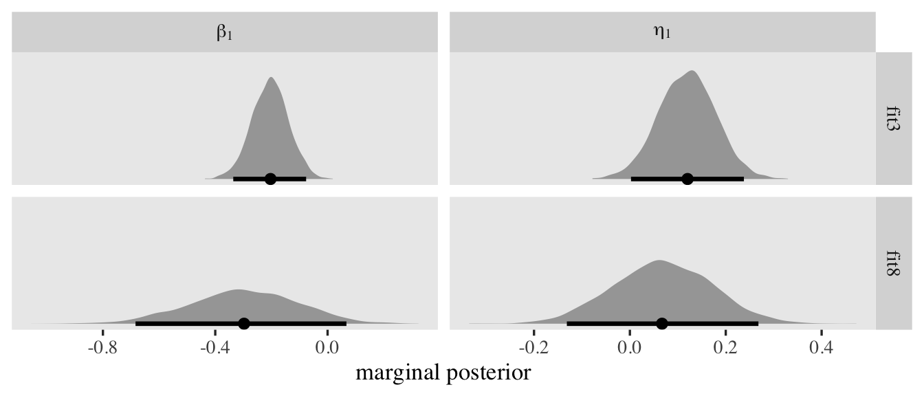
For my money, the posteriors from the conditional distributional model fit8 are more valid than those from the highly-constrained fit3. Now that male is back in the game, let’s plot the latent distributions again.

tibble(male  = 0:1,
       mu    = c(0, fixef(fit8)["male", 1]),
       sigma = 1 / exp(c(0, fixef(fit8)["disc_male", 1]))) %>% 
  expand(nesting(male, mu, sigma),
         x = seq(from = -3.5, to = 3.5, length.out = 200)) %>% 
  mutate(d   = dnorm(x, mean = mu, sd = sigma),
         sex = ifelse(male == 0, "female", "male")) %>% 
  
  ggplot(aes(x = x, y = d, fill = sex)) +
  geom_area(alpha = 1/2, position = "identity") +
  scale_fill_manual(NULL, values = c("red3", "blue3")) +
  scale_x_continuous(expression(Phi), breaks = -3:3) +
  scale_y_continuous(NULL, breaks = NULL) +
  labs(title = "Latent distributions for fit8",
       subtitle = expression("The shape for men is based on the posterior means of the "*beta[1]*" and "*eta[1]*" parameters.")) +
  coord_cartesian(xlim = c(-3, 3)) +
  theme(panel.grid = element_blank())

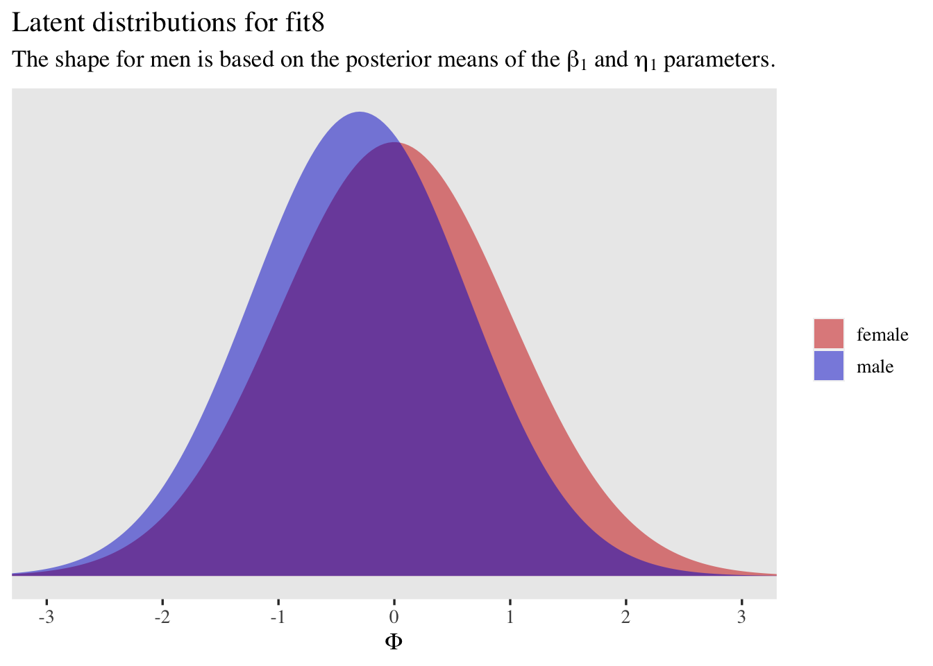
Unlike with the previous latent density plots, we have left out the threshold lines for this one. With \(25\) \(\tau_{kj}\) parameters, showing them all would just clutter things up. But since we now our latent \(\mu\) and \(\sigma\) parameters vary across all \(200\) participants, it might be fun to visualize those.

d %>% 
  distinct(id, male) %>% 
  mutate(beta0 = 0,
         beta1 = fixef(fit8)["male", 1],
         u_i = ranef(fit8)$id[, 1, "Intercept"],
         eta0 = 0,
         eta1 = fixef(fit8)["disc_male", 1],
         w_i = ranef(fit8)$id[, 1, "disc_Intercept"]) %>% 
  mutate(mu_i = beta0 + beta1 * male + u_i,
         sigma_i = 1 / exp(eta0 + eta1 * male + w_i)) %>% 
  expand(nesting(id, male, mu_i, sigma_i),
         x = seq(from = -6.5, to = 6.5, length.out = 200)) %>% 
  mutate(d   = dnorm(x, mean = mu_i, sd = sigma_i),
         sex = ifelse(male == 0, "female", "male")) %>% 
  # unnecessary, but keeps male on the left, which matches the position of the previous plot
  mutate(sex = fct_rev(sex)) %>% 
  
  ggplot(aes(x = x, y = d, fill = sex, color = sex, group = id)) +
  geom_area(alpha = 1/20, linewidth = 1/20, position = "identity") +
  scale_fill_manual(values = c("blue3", "red3"), breaks = NULL) +
  scale_color_manual(values = c("blue3", "red3"), breaks = NULL) +
  scale_x_continuous(expression(Phi), breaks = -3:3 * 2) +
  scale_y_continuous(NULL, breaks = NULL) +
  labs(title = "Person-level latent distributions for fit8",
       subtitle = expression("The shapes are based on the posterior means of the "*beta[1]*", "*eta[1]*", "*italic(u[i])*", and "*italic(w[i])*" parameters.")) +
  coord_cartesian(xlim = c(-5.7, 5.7)) +
  theme(panel.grid = element_blank()) +
  facet_wrap(~ sex)

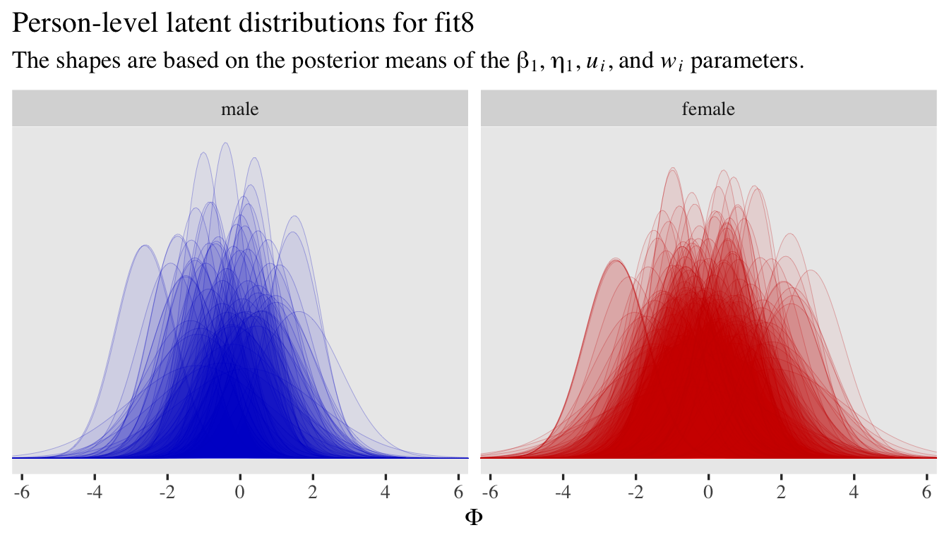
As this is a fully cross-classified model, we can make a similar plot for the question-level latent densities.

d %>% 
  distinct(item) %>% 
  mutate(beta0 = 0,
         beta1 = fixef(fit8)["male", 1],
         v_i = ranef(fit8)$item[, 1, "Intercept"],
         eta0 = 0,
         eta1 = fixef(fit8)["disc_male", 1],
         x_i = ranef(fit8)$item[, 1, "disc_Intercept"]) %>% 
  expand(nesting(item, beta0, beta1, v_i, eta0, eta1, x_i),
         male = 0:1) %>% 
  mutate(mu_j = beta0 + beta1 * male + v_i,
         sigma_j = 1 / exp(eta0 + eta1 * male + x_i)) %>% 
  expand(nesting(item, male, mu_j, sigma_j),
         x = seq(from = -5, to = 5, length.out = 200)) %>% 
  mutate(d   = dnorm(x, mean = mu_j, sd = sigma_j),
         sex = ifelse(male == 0, "female", "male")) %>% 
  # unnecessary, but keeps male on the left, which matches the position of the previous plots
  mutate(sex = fct_rev(sex)) %>% 
  
  ggplot(aes(x = x, y = d, fill = item, color = item, group = item)) +
  geom_area(alpha = 1/4, linewidth = 1/2, position = "identity") +
  
  scale_fill_viridis_d(NULL, option = "A", end = 0.85, direction = -1) +
  scale_color_viridis_d(NULL, option = "A", end = 0.85, direction = -1) +
  scale_x_continuous(expression(Phi), breaks = -2:2 * 2) +
  scale_y_continuous(NULL, breaks = NULL) +
  labs(title = "Question-level latent distributions for fit8",
       subtitle = expression("The shapes are based on the posterior means of the "*beta[1]*", "*eta[1]*", "*italic(v[j])*", and "*italic(x[j])*" parameters.")) +
  coord_cartesian(xlim = c(-4.25, 4.25)) +
  theme(panel.grid = element_blank()) +
  facet_wrap(~ sex) 

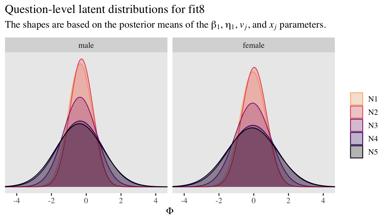
Even though you might think of male as a person-level variable, you still need to account for it when plotting the question-level distributions because the grand-mean values for \(\mu\) and \(\sigma\) are both conditional on male.

Do bear in mind, though, that the latent means and spreads the items share a very tenuous relationship with the naïve sample statistics.

d %>%
  mutate(sex = ifelse(male == 0, "female", "male")) %>%
  # unnecessary, but keeps male on the left, which matches the position of the previous plots
  mutate(sex = fct_rev(sex)) %>%
  group_by(sex, item) %>%
  summarise(m = mean(rating),
            s = sd(rating)) %>%
  mutate_if(is.double, round, digits = 1) %>%
  mutate(stat = str_c(m, " (", s, ")")) %>%
  select(-m, -s) %>%
  pivot_wider(names_from = sex, values_from = stat)

## # A tibble: 5 × 3
##   item  male      female   
##   <chr> <chr>     <chr>    
## 1 N1    3.1 (1.5) 3.1 (1.6)
## 2 N2    3.4 (1.4) 3.5 (1.6)
## 3 N3    2.8 (1.3) 3.3 (1.7)
## 4 N4    3.2 (1.6) 3.3 (1.5)
## 5 N5    2.3 (1.4) 3.4 (1.6)

I believe this apparent mismatch is because of how the cumulative probit model uses thresholds and the normal CDF to describe relative probabilities among the ordinal categories. The latent means and standard deviations have very different meanings from the sample statistics. So it goes…

From an IRT perspective, we can think of the \(\mu_j\) and \(\alpha_j\) parameters as item difficulty and discrimination parameters. Here we display them in a coefficient plot in the same way seen in Figure \(10\) in Bürkner’s IRT ( 2020) tutorial.

rbind(ranef(fit8)$item[, , "Intercept"],
      ranef(fit8)$item[, , "disc_Intercept"] %>% exp()) %>% 
  data.frame() %>% 
  mutate(item = rep(str_c("N", 1:5), times = 2),
         parameter = rep(c("difficulty", "discrimination"), each = 5)) %>% 
  
  ggplot(aes(x = Estimate, xmin = Q2.5, xmax = Q97.5, y = item)) +
  geom_pointrange(fatten = 1.5) +
  labs(title = "IRT-based item parameters for fit8",
       x = "marginal posterior") +
  facet_wrap(~ parameter)

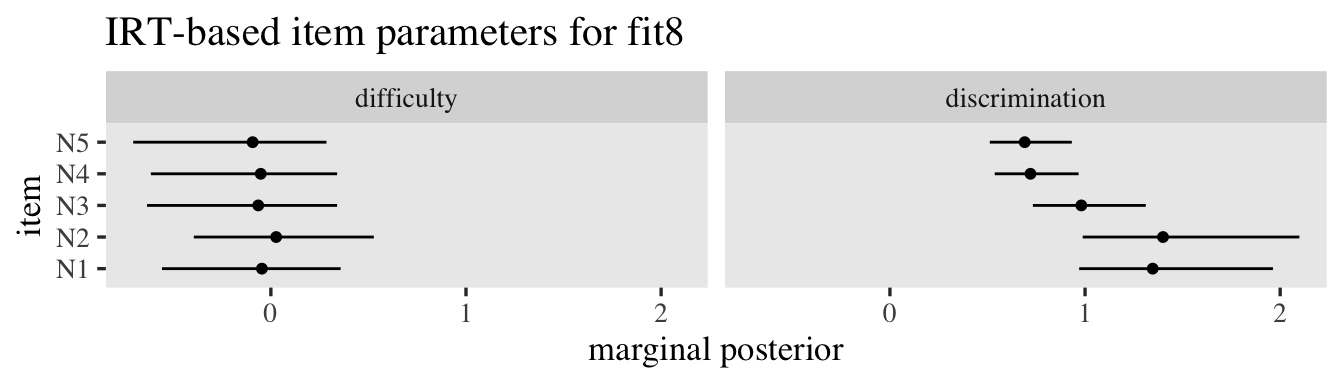
I still haven’t figured out how to make item-characteristic curves for an ordinal model. If you know how, please chime in on twitter. And that last plot’s going to wrap this little blog post up. If you have any concerns about my equations or the workflows, herein, do chime in to twitter. This is a resource for us all and I’d hate to spread incorrect methods.

New blog up!https://t.co/6T08AY8VDJ

Some of my recent projects required the Bayesian cumulative probit model. To bet a better handle on the cumulative probit, I worked through some toy problems. This blog contains my notes.

If you see errors, do chime in.#brms

— Solomon Kurz (@SolomonKurz) December 30, 2021

Happy modeling, friends.

Session info

sessionInfo()

## R version 4.2.0 (2022-04-22)
## Platform: x86_64-apple-darwin17.0 (64-bit)
## Running under: macOS Big Sur/Monterey 10.16
## 
## Matrix products: default
## BLAS:   /Library/Frameworks/R.framework/Versions/4.2/Resources/lib/libRblas.0.dylib
## LAPACK: /Library/Frameworks/R.framework/Versions/4.2/Resources/lib/libRlapack.dylib
## 
## locale:
## [1] en_US.UTF-8/en_US.UTF-8/en_US.UTF-8/C/en_US.UTF-8/en_US.UTF-8
## 
## attached base packages:
## [1] stats     graphics  grDevices utils     datasets  methods   base     
## 
## other attached packages:
##  [1] tidybayes_3.0.2 brms_2.18.0     Rcpp_1.0.9      forcats_0.5.1   stringr_1.4.1   dplyr_1.0.10    purrr_0.3.4    
##  [8] readr_2.1.2     tidyr_1.2.1     tibble_3.1.8    ggplot2_3.4.0   tidyverse_1.3.2
## 
## loaded via a namespace (and not attached):
##   [1] readxl_1.4.1         backports_1.4.1      plyr_1.8.7           igraph_1.3.4         svUnit_1.0.6        
##   [6] splines_4.2.0        crosstalk_1.2.0      TH.data_1.1-1        rstantools_2.2.0     inline_0.3.19       
##  [11] digest_0.6.30        htmltools_0.5.3      viridis_0.6.2        fansi_1.0.3          magrittr_2.0.3      
##  [16] checkmate_2.1.0      googlesheets4_1.0.1  tzdb_0.3.0           modelr_0.1.8         RcppParallel_5.1.5  
##  [21] matrixStats_0.62.0   xts_0.12.1           sandwich_3.0-2       prettyunits_1.1.1    colorspace_2.0-3    
##  [26] rvest_1.0.2          ggdist_3.2.0         haven_2.5.1          xfun_0.35            callr_3.7.3         
##  [31] crayon_1.5.2         jsonlite_1.8.3       lme4_1.1-31          survival_3.4-0       zoo_1.8-10          
##  [36] glue_1.6.2           gtable_0.3.1         gargle_1.2.0         emmeans_1.8.0        distributional_0.3.1
##  [41] pkgbuild_1.3.1       rstan_2.21.7         abind_1.4-5          scales_1.2.1         mvtnorm_1.1-3       
##  [46] DBI_1.1.3            miniUI_0.1.1.1       viridisLite_0.4.1    xtable_1.8-4         diffobj_0.3.5       
##  [51] stats4_4.2.0         StanHeaders_2.21.0-7 DT_0.24              htmlwidgets_1.5.4    httr_1.4.4          
##  [56] threejs_0.3.3        arrayhelpers_1.1-0   posterior_1.3.1      ellipsis_0.3.2       pkgconfig_2.0.3     
##  [61] loo_2.5.1            farver_2.1.1         sass_0.4.2           dbplyr_2.2.1         utf8_1.2.2          
##  [66] labeling_0.4.2       tidyselect_1.1.2     rlang_1.0.6          reshape2_1.4.4       later_1.3.0         
##  [71] munsell_0.5.0        cellranger_1.1.0     tools_4.2.0          cachem_1.0.6         cli_3.4.1           
##  [76] generics_0.1.3       broom_1.0.1          ggridges_0.5.3       evaluate_0.18        fastmap_1.1.0       
##  [81] yaml_2.3.5           processx_3.8.0       knitr_1.40           fs_1.5.2             nlme_3.1-159        
##  [86] mime_0.12            projpred_2.2.1       xml2_1.3.3           compiler_4.2.0       bayesplot_1.9.0     
##  [91] shinythemes_1.2.0    rstudioapi_0.13      gamm4_0.2-6          reprex_2.0.2         bslib_0.4.0         
##  [96] stringi_1.7.8        highr_0.9            ps_1.7.2             blogdown_1.15        Brobdingnag_1.2-8   
## [101] lattice_0.20-45      Matrix_1.4-1         psych_2.2.5          nloptr_2.0.3         markdown_1.1        
## [106] shinyjs_2.1.0        tensorA_0.36.2       vctrs_0.5.0          pillar_1.8.1         lifecycle_1.0.3     
## [111] jquerylib_0.1.4      bridgesampling_1.1-2 estimability_1.4.1   httpuv_1.6.5         R6_2.5.1            
## [116] bookdown_0.28        promises_1.2.0.1     gridExtra_2.3        codetools_0.2-18     boot_1.3-28         
## [121] colourpicker_1.1.1   MASS_7.3-58.1        gtools_3.9.3         assertthat_0.2.1     withr_2.5.0         
## [126] mnormt_2.1.0         shinystan_2.6.0      multcomp_1.4-20      mgcv_1.8-40          parallel_4.2.0      
## [131] hms_1.1.1            grid_4.2.0           coda_0.19-4          minqa_1.2.5          rmarkdown_2.16      
## [136] googledrive_2.0.0    shiny_1.7.2          lubridate_1.8.0      base64enc_0.1-3      dygraphs_1.1.1.6

References

Bürkner, P.-C. (2020). Bayesian item response modeling in R with brms and Stan. http://arxiv.org/abs/1905.09501
Bürkner, P.-C. (2017). brms: An R package for Bayesian multilevel models using Stan. Journal of Statistical Software, 80(1), 1–28. https://doi.org/10.18637/jss.v080.i01
Bürkner, P.-C. (2018). Advanced Bayesian multilevel modeling with the R package brms. The R Journal, 10(1), 395–411. https://doi.org/10.32614/RJ-2018-017
Bürkner, P.-C. (2022). brms: Bayesian regression models using ’Stan’. https://CRAN.R-project.org/package=brms
Efron, B., & Morris, C. (1977). Stein’s paradox in statistics. Scientific American, 236(5), 119–127. https://doi.org/10.1038/scientificamerican0577-119
Goldberg, L. R. (1999). A broad-bandwidth, public domain, personality inventory measuring the lower-level facets of several five-factor models. In I. Mervielde, I. Deary, F. De Fruyt, & F. Ostendorf (Eds.), Personality psychology in Europe (Vol. 7, pp. 7–28). Tilburg University Press.
Kay, M. (2022). tidybayes: Tidy data and ’geoms’ for Bayesian models. https://CRAN.R-project.org/package=tidybayes
Kruschke, J. K. (2015). Doing Bayesian data analysis: A tutorial with R, JAGS, and Stan. Academic Press. https://sites.google.com/site/doingbayesiandataanalysis/
Kurz, A. S. (2020a). Doing Bayesian data analysis in brms and the tidyverse (version 0.4.0). https://bookdown.org/content/3686/
Kurz, A. S. (2020b). Statistical rethinking with brms, ggplot2, and the tidyverse (version 1.2.0). https://doi.org/10.5281/zenodo.3693202
McElreath, R. (2020). Statistical rethinking: A Bayesian course with examples in R and Stan (Second Edition). CRC Press. https://xcelab.net/rm/statistical-rethinking/
McElreath, R. (2015). Statistical rethinking: A Bayesian course with examples in R and Stan. CRC press. https://xcelab.net/rm/statistical-rethinking/
R Core Team. (2022). R: A language and environment for statistical computing. R Foundation for Statistical Computing. https://www.R-project.org/
Revelle, W. (2022). psych: Procedures for psychological, psychometric, and personality research. https://CRAN.R-project.org/package=psych
Revelle, W., Wilt, J., & Rosenthal, A. (2010). Individual differences in cognition: New methods for examining the personality-cognition link. In A. Gruszka, G. Matthews, & B. Szymura (Eds.), Handbook of individual differences in cognition: Attention, memory and executive control (pp. 27–49). Springer.
Wickham, H. (2022). tidyverse: Easily install and load the ’tidyverse’. https://CRAN.R-project.org/package=tidyverse
Wickham, H., Averick, M., Bryan, J., Chang, W., McGowan, L. D., François, R., Grolemund, G., Hayes, A., Henry, L., Hester, J., Kuhn, M., Pedersen, T. L., Miller, E., Bache, S. M., Müller, K., Ooms, J., Robinson, D., Seidel, D. P., Spinu, V., … Yutani, H. (2019). Welcome to the tidyverse. Journal of Open Source Software, 4(43), 1686. https://doi.org/10.21105/joss.01686
- Posted on:
- December 29, 2021
- Length:
- 70 minute read, 14712 words