Stein's Paradox and What Partial Pooling Can Do For You
By A. Solomon Kurz
February 23, 2019
[edited on January 18, 2021]
tl;dr
Sometimes a mathematical result is strikingly contrary to generally held belief even though an obviously valid proof is given. Charles Stein of Stanford University discovered such a paradox in statistics in 1955. His result undermined a century and a half of work on estimation theory. ( Efron & Morris, 1977, p. 119) The James-Stein estimator leads to better predictions than simple means. Though I don’t recommend you actually use the James-Stein estimator in applied research, understanding why it works might help clarify why it’s time social scientists consider defaulting to multilevel models for their work-a-day projects.
The James-Stein can help us understand multilevel models.
I recently noticed someone—I wish I could recall who—tweet about Efron and Morris’s classic paper, Stein’s paradox in statistics. At the time, I was vaguely aware of the paper but hadn’t taken the chance to read it. The tweet’s author mentioned how good a read it was. Now I’ve finally given it a look, I concur. I’m not a sports fan, but I really appreciated their primary example using batting averages from baseball players in 1970. It clarified why partial pooling leads to better estimates than taking simple averages.
In this post, I’ll walk out Efron and Morris’s baseball example and then link it to contemporary Bayesian multilevel models.
I assume things.
For this project, I’m presuming you are familiar with logistic regression, vaguely familiar with the basic differences between frequentist and Bayesian approaches to fitting regression models, and have heard of multilevel models. All code in is R ( R Core Team, 2022), with a heavy use of the tidyverse ( Wickham et al., 2019; Wickham, 2022), and the brms package for Bayesian regression ( Bürkner, 2017, 2018, 2022).
Behold the baseball data.
Stein’s paradox concerns the use of observed averages to estimate unobservable quantities. Averaging is the second most basic process in statistics, the first being the simple act of counting. A baseball player who gets seven hits in 20 official times at bat is said to have a batting average of .350. In computing this statistic we are forming an estimate of the payer’s true batting ability in terms of his observed average rate of success. Asked how well the player will do in his next 100 times at bat, we would probably predict 35 more hits. In traditional statistical theory it can be proved that no other estimation rule is uniformly better than the observed average.
The paradoxical element in Stein’s result is that it sometimes contradicts this elementary law of statistical theory. If we have three or more baseball players, and if we are interested in predicting future batting averages for each of them, then there is a procedure that is better than simply extrapolating from the three separate averages…
As our primary data we shall consider the batting averages of 18 major-league players as they were recorded after their first 45 times at bat in the 1970 season. ( Efron & Morris, 1977, p. 119) Let’s enter the
baseballdata.
library(tidyverse)
baseball <-
  tibble(player = c("Clemente", "F Robinson", "F Howard", "Johnstone", "Berry", "Spencer", "Kessinger", "L Alvarado", "Santo", "Swoboda", "Unser", "Williams", "Scott", "Petrocelli", "E Rodriguez", "Campaneris", "Munson", "Alvis"),
         hits = c(18:15, 14, 14:12, 11, 11, rep(10, times = 5), 9:7),
         times_at_bat = 45,
         true_ba = c(.346, .298, .276, .222, .273, .27, .263, .21, .269, .23, .264, .256, .303, .264, .226, .286, .316, .2))
Here’s what those data look like.
glimpse(baseball)
## Rows: 18
## Columns: 4
## $ player       <chr> "Clemente", "F Robinson", "F Howard", "Johnstone", "Berry", "Spencer", "Kessi…
## $ hits         <dbl> 18, 17, 16, 15, 14, 14, 13, 12, 11, 11, 10, 10, 10, 10, 10, 9, 8, 7
## $ times_at_bat <dbl> 45, 45, 45, 45, 45, 45, 45, 45, 45, 45, 45, 45, 45, 45, 45, 45, 45, 45
## $ true_ba      <dbl> 0.346, 0.298, 0.276, 0.222, 0.273, 0.270, 0.263, 0.210, 0.269, 0.230, 0.264, …
We have data from 18 players. The main columns are of the number of hits for their first 45 times_at_bat. I got the player, hits, and times_at_bat values directly from the paper. However, Efron and Morris didn’t include the batting averages for the end of the season in the paper. Happily, I was able to find those values in the
online posting of the first chapter of one of Effron’s books (
2010) . They’re included in the true_ba column.
These were all the players who happened to have batted exactly 45 times the day the data were tabulated. A batting average is defined, of course, simply as the number of hits divided by the number of times at bat; it is always a number between 0 and 1. ( Efron & Morris, 1977, p. 119) I like use a lot of plots to better understand what I’m doing. Before we start plotting, I should point out the color theme in this project comes from here. [Haters gonna hate.]
navy_blue <- "#0C2C56"
nw_green  <- "#005C5C"
silver    <- "#C4CED4"
theme_set(theme_grey() +
            theme(panel.grid = element_blank(),
                  panel.background = element_rect(fill = silver),
                  strip.background = element_rect(fill = silver)))
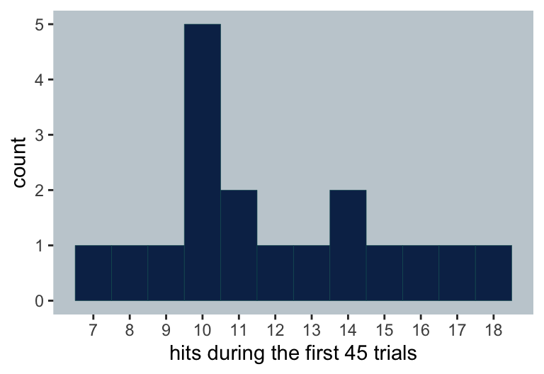
We might use a histogram to get a sense of the hits.
baseball %>%
  ggplot(aes(x = hits)) +
  geom_histogram(color = nw_green,
                 fill  = navy_blue,
                 size  = 1/10, binwidth = 1) +
  scale_x_continuous("hits during the first 45 trials",
                     breaks = 7:18)
## Warning: Using `size` aesthetic for lines was deprecated in ggplot2 3.4.0.
## ℹ Please use `linewidth` instead.
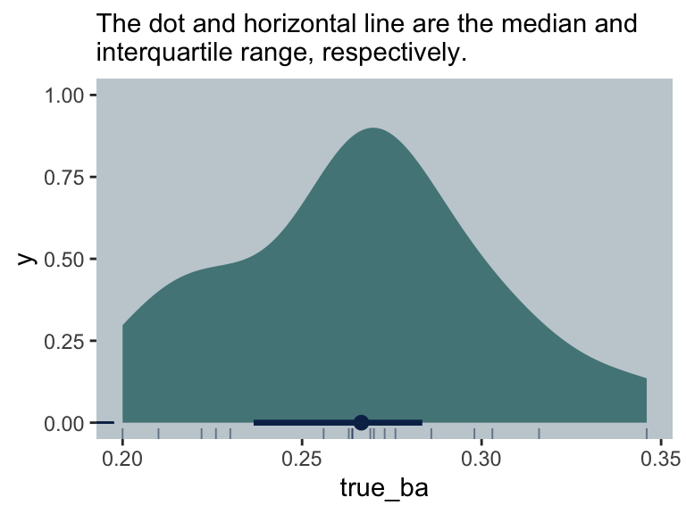
Here is the distribution of the end-of-the-season batting averages, true_ba.
library(tidybayes)
baseball %>%
  ggplot(aes(x = true_ba, y = 0)) +
  stat_halfeye(point_interval = median_qi, .width = .5,
               color = navy_blue, fill = alpha(nw_green, 2/3)) +
  geom_rug(color = navy_blue, size = 1/3, alpha = 1/2) +
  ggtitle(NULL,
          subtitle = "The dot and horizontal line are the median and\ninterquartile range, respectively.")
James-Stein will help us achieve our goal.
For each of the 18 players in the data, our goal is to the best job possible to use the data for their first 45 times at bat (i.e., hits and times_at_bat) to predict their batting averages at the end of the season (i.e., true_ba). Before Charles Stein, the conventional reasoning was their initial batting averages (i.e., hits / times_at_bat) are the best way to do this. It turns out that would be naïve. To see why, let
y(i.e.,\(y\)) = the batting average for the first 45 times at bat,y_bar(i.e.,\(\overline y\)) = the grand mean for the first 45 times at bat,c(i.e.,\(c\)) = shrinking factor,z(i.e.,\(z\)) = James-Stein estimate, andtrue_ba(i.e.,theta,\(\theta\)) = the batting average at the end of the season.
The first step in applying Stein’s method is to determine the average of the averages. Obviously this grand average, which we give the symbol
\(\overline y\), must also lie between 0 and 1. The essential process in Stein’s method is the “shrinking” of all the individual averages toward this grand average. If a player’s hitting record is better than the grand average, then it must be reduced; if he is not hitting as well as the grand average, then his hitting record must be increased. The resulting shrunken value for each player we designate\(z\). ( Efron & Morris, 1977, p. 119) As such, the James-Stein estimator is
$$z = \overline y + c(y - \overline y),$$
where, in the paper, \(c = .212\). Let’s get some of those values into the baseball data.
(
  baseball <-
  baseball %>%
  mutate(y = hits / times_at_bat) %>%
  mutate(y_bar = mean(y),
         c     = .212) %>%
  mutate(z     = y_bar + c * (y - y_bar),
         theta = true_ba)
  )
## # A tibble: 18 × 9
##    player       hits times_at_bat true_ba     y y_bar     c     z theta
##    <chr>       <dbl>        <dbl>   <dbl> <dbl> <dbl> <dbl> <dbl> <dbl>
##  1 Clemente       18           45   0.346 0.4   0.265 0.212 0.294 0.346
##  2 F Robinson     17           45   0.298 0.378 0.265 0.212 0.289 0.298
##  3 F Howard       16           45   0.276 0.356 0.265 0.212 0.285 0.276
##  4 Johnstone      15           45   0.222 0.333 0.265 0.212 0.280 0.222
##  5 Berry          14           45   0.273 0.311 0.265 0.212 0.275 0.273
##  6 Spencer        14           45   0.27  0.311 0.265 0.212 0.275 0.27
##  7 Kessinger      13           45   0.263 0.289 0.265 0.212 0.270 0.263
##  8 L Alvarado     12           45   0.21  0.267 0.265 0.212 0.266 0.21
##  9 Santo          11           45   0.269 0.244 0.265 0.212 0.261 0.269
## 10 Swoboda        11           45   0.23  0.244 0.265 0.212 0.261 0.23
## 11 Unser          10           45   0.264 0.222 0.265 0.212 0.256 0.264
## 12 Williams       10           45   0.256 0.222 0.265 0.212 0.256 0.256
## 13 Scott          10           45   0.303 0.222 0.265 0.212 0.256 0.303
## 14 Petrocelli     10           45   0.264 0.222 0.265 0.212 0.256 0.264
## 15 E Rodriguez    10           45   0.226 0.222 0.265 0.212 0.256 0.226
## 16 Campaneris      9           45   0.286 0.2   0.265 0.212 0.252 0.286
## 17 Munson          8           45   0.316 0.178 0.265 0.212 0.247 0.316
## 18 Alvis           7           45   0.2   0.156 0.265 0.212 0.242 0.2
Which set of values,
\(y\)or\(z\), is the better indicator of batting ability for the 18 players in our example? In order to answer that question in a precise way one would have to know the “true batting ability” of each player. This true average we shall designate\(\theta\)(the Greek letter theta). Actually it is an unknowable quantity, an abstraction representing the probability that a player will get a hit on any given time at bat. Although\(\theta\)is unobservable, we have a good approximation to it: the subsequent performance of the batters. It is sufficient to consider just the remainder of the 1970 season, which includes about nine times as much data as the preliminary averages were based on. ( Efron & Morris, 1977, p. 119) Now we have both\(y\)and\(z\)in the data, let’s compare their distributions.
baseball %>%
  pivot_longer(cols = c(y, z)) %>%
  mutate(label = ifelse(name == "z",
                        "the James-Stein estimate",
                        "early-season batting average")) %>%

  ggplot(aes(x = value, y = label)) +
  geom_vline(xintercept = 0.2654321, linetype = 2,
             color = "white") +
  stat_halfeye(point_interval = median_qi, .width = .5,
               color = navy_blue, fill = alpha(nw_green, 2/3),
               height = 4) +
  labs(x = "batting average", y = NULL) +
  coord_cartesian(ylim = c(1.25, 5.25))
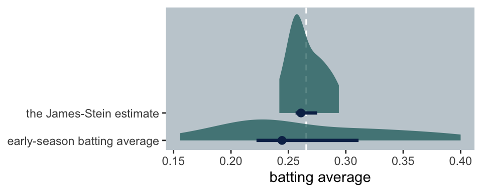
As implied in the formula, the James-Stein estimates are substantially shrunken towards the grand mean, y_bar. To get a sense of which estimate is better, we can subtract the estimate from theta, the end of the season batting average.
baseball <-
  baseball %>%
  mutate(y_error = theta - y,
         z_error = theta - z)
Since y_error and y_error are error distributions, we prefer values to be as close to zero as possible. Let’s take a look.
baseball %>%
  pivot_longer(y_error:z_error) %>%

  ggplot(aes(x = value, y = name)) +
  geom_vline(xintercept = 0, linetype = 2,
             color = "white") +
  stat_halfeye(point_interval = median_qi, .width = .5,
               color = navy_blue, fill = alpha(nw_green, 2/3),
               height = 2.5) +
  labs(x = NULL, y = NULL) +
  coord_cartesian(ylim = c(1.25, 4))
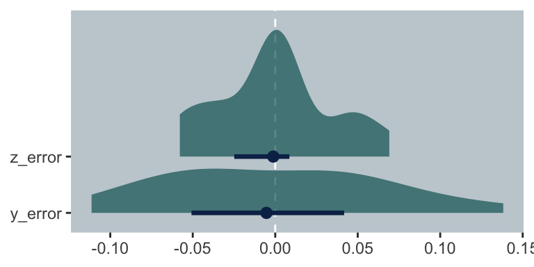
The James-Stein errors (i.e., z_error) are more concentrated toward zero. In the paper, we read: “One method of evaluating the two estimates is by simply counting their successes and failures. For 16 of the 18 players the James-Stein estimator \(z\) is closer than the observed average \(y\) to the ‘true,’ or seasonal, average \(\theta\)” (pp. 119–121). We can compute that with a little ifelse().
baseball %>%
  transmute(closer_to_theta = ifelse(abs(y_error) - abs(z_error) == 0, "equal",
                                     ifelse(abs(y_error) - abs(z_error) > 0, "z", "y"))) %>%
  count(closer_to_theta)
## # A tibble: 2 × 2
##   closer_to_theta     n
##   <chr>           <int>
## 1 y                   2
## 2 z                  16
A more quantitative way of comparing the two techniques is through the total squared error of estimation… The observed averages
\(y\)have a total squared error of .077, whereas the squared error of the James-Stein estimators is only .022. By this comparison, then, Stein’s method is 3.5 times as accurate. ( Efron & Morris, 1977, p. 121)
baseball %>%
  pivot_longer(y_error:z_error) %>%
  group_by(name) %>%
  summarise(total_squared_error = sum(value * value))
## # A tibble: 2 × 2
##   name    total_squared_error
##   <chr>                 <dbl>
## 1 y_error              0.0755
## 2 z_error              0.0214
We can get the 3.5 value with simple division.
0.07548795 / 0.02137602
## [1] 3.531431
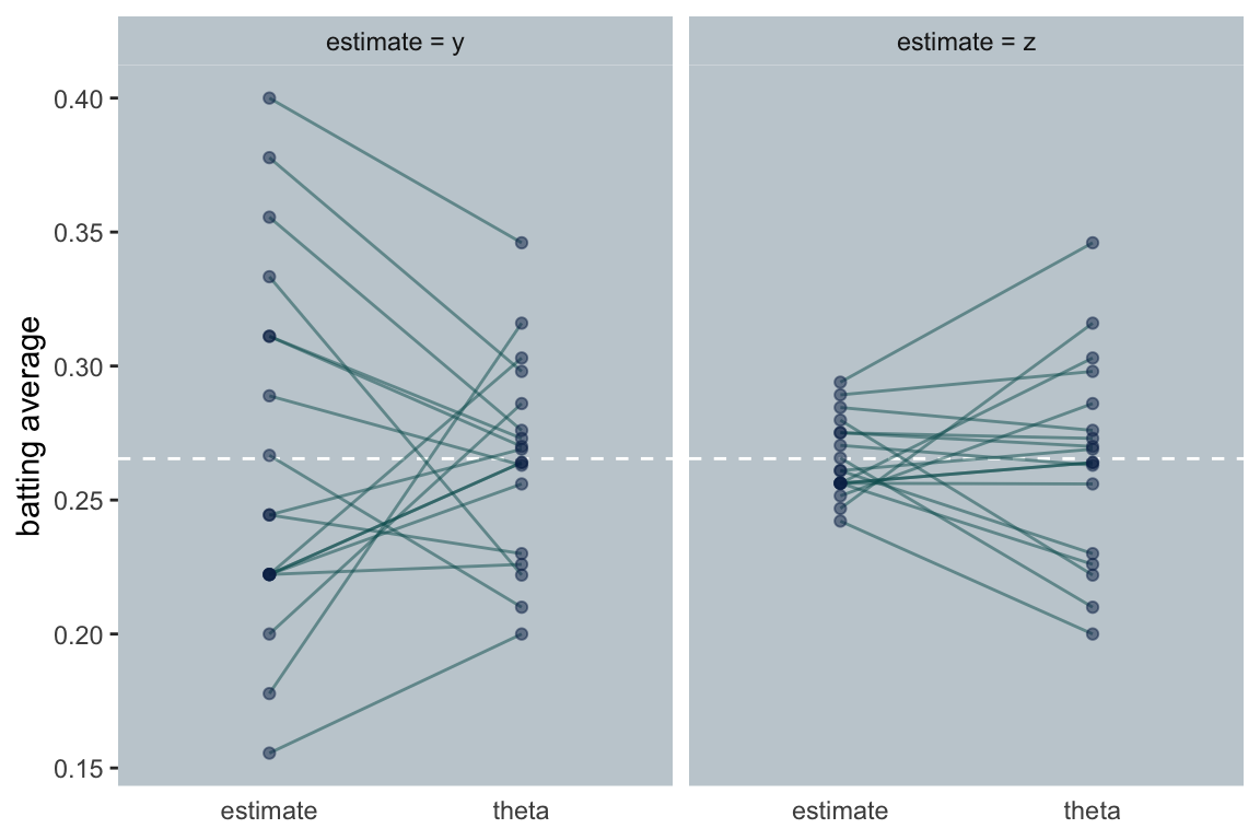
So it does indeed turn out that shrinking each player’s initial estimate toward the grand mean of those initial estimates does a better job of predicting their end-of-the-season batting averages than using their individual batting averages. To get a sense of what this looks like, let’s make our own version of the figure on page 121.
bind_rows(
  baseball %>%
    select(y, z, theta, player) %>%
    gather(key, value, -player) %>%
    mutate(time = ifelse(key == "theta", "theta", "estimate")),
  baseball %>%
    select(player, theta) %>%
    rename(value = theta) %>%
    mutate(key  = "theta",
           time = "theta")
) %>%
  mutate(facet = rep(c("estimate = y", "estimate = z"), each = n() / 4) %>% rep(., times = 2)) %>%

  ggplot(aes(x = time, y = value, group = player)) +
  geom_hline(yintercept = 0.2654321, linetype = 2,
             color = "white") +
  geom_line(alpha = 1/2,
            color = nw_green) +
  geom_point(alpha = 1/2,
             color = navy_blue) +
  labs(x = NULL,
       y = "batting average") +
  theme(axis.ticks.x = element_blank()) +
  facet_wrap(~facet)
The James-Stein estimator works because of its shrinkage, and the shrinkage factor is called \(c\). Though in the first parts of the paper, Efron and Morris just told us \(c = .212\), they gave the actual formula for \(c\) a little later on. If you let \(k\) be the number of means (i.e., the number of clusters), then
$$c = 1 - \frac{(k - 3)\sigma^2}{\sum (y - \overline y)^2}.$$
The difficulty of that formula is we don’t know the value for \(\sigma^2\). It’s not the sample variance of \(y\) (i.e., var(y)). An
answer to this stackexchange question helped clarify Efron and Morris were using the formula for the standard error of the estimate,
$$\sqrt{\hat p(1 - \hat p) / n},$$
which, in the variance metric, is simply
$$\hat p(1 - \hat p) / n.$$
Following along, we can compute sigma_squared like so:
(sigma_squared <- mean(baseball$y) * (1 - mean(baseball$y)) / 45)
## [1] 0.004332842
Now we can reproduce the \(c\) value from the paper.
baseball %>%
  select(player, y:c) %>%
  mutate(squared_deviation = (y - y_bar)^2) %>%
  summarise(c_by_hand = 1 - ((n() - 3) * sigma_squared / sum(squared_deviation)))
## # A tibble: 1 × 1
##   c_by_hand
##       <dbl>
## 1     0.212
Let’s go Bayesian.
This has been fun. But I don’t recommend you actually use the James-Stein estimator in your research.
The James-Stein estimator is not the only one that is known to be better than the sample averages…
The search for new estimators continues. Recent efforts [in the 1970s, that is] have been concentrated on achieving results like those obtained with Stein’s method for problems involving distributions other than the normal distribution. Several lines of work, including Stein’s and Robbins’ and more formal Bayesian methods seem to be converging on a powerful general theory of parameter estimation. ( Efron & Morris, 1977, p. 127, emphasis added) The James-Stein estimator is not Bayesian, but it is a precursor to the kind of analyses we now do with Bayesian multilevel models, which pool cluster-level means toward a grand mean. To get a sense of this, we’ll fit a couple models. First, let’s load the brms package.
library(brms)
I typically work with the linear regression paradigm. If we were to analyze the baseball data, we’d use an aggregated binomial mode, which is a particular kind of logistic regression. You can learn more about it
here. If we wanted a model that corresponded to the \(y\) estimates, above, we’d use hits as the criterion and allow each player to get his own separate estimate. Since we’re working within the Bayesian paradigm, we also need to assign priors. In this case, we’ll use a weakly-regularizing \(\operatorname{Normal}(0, 1.5)\) on the intercepts. See
this wiki for more on weakly-regularizing priors.
Here’s the code to fit the model with brms.
fit_y <-
  brm(data = baseball,
      family = binomial,
      hits | trials(45) ~ 0 + player,
      prior(normal(0, 1.5), class = b),
      seed = 1)
If you were curious, that model followed the statistical formula
$$
\begin{align*} \text{hits}_i & \sim \operatorname{Binomial} (n = 45, p_i) \\ \operatorname{logit}(p_i) & = \alpha_\text{player} \\ \alpha_\text{player} & \sim \operatorname{Normal}(0, 1.5), \end{align*}
$$
where \(p_i\) is the probability of player \(i\), \(\alpha_\text{player}\) is a vector of \(\text{player}\)-specific intercepts from within the logistic regression model, and each of those intercepts are given a \(\operatorname{Normal}(0, 1.5)\) prior on the log-odds scale. (If this is all new and confusing, don’t worry. I’ll recommended some resources at the end of this post.)
For our analogue to the James-Stein estimate \(z\), we’ll fit the multilevel version of that last model. While each player still gets his own estimate, those estimates are now partially-pooled toward the grand mean.
fit_z <-
  brm(data = baseball,
      family = binomial,
      hits | trials(45) ~ 1 + (1 | player),
      prior = c(prior(normal(0, 1.5), class = Intercept),
                prior(normal(0, 1.5), class = sd)),
      seed = 1)
That model followed the statistical formula
$$
\begin{align*} \text{hits}_i & \sim \operatorname{Binomial}(n = 45, p_i) \\ \operatorname{logit}(p_i) & = \alpha + \alpha_\text{player} \\ \alpha & \sim \operatorname{Normal}(0, 1.5) \\ \alpha_\text{player} & \sim \operatorname{Normal}(0, \sigma_\text{player}) \\ \sigma_\text{player} & \sim \operatorname{HalfNormal}(0, 1.5), \end{align*}
$$
where \(\alpha\) is the grand mean among the \(\text{player}\)-specific intercepts, \(\alpha_\text{player}\) is the vector of \(\text{player}\)-specific deviations from the grand mean, which are Normally distributed with a mean of zero and a standard deviation of \(\sigma_\text{player}\), which is estimated from the data.
Here are the model summaries.
fit_y$fit
## Inference for Stan model: 66daca5fdbbf7ebccc1bfc693007bd14.
## 4 chains, each with iter=2000; warmup=1000; thin=1;
## post-warmup draws per chain=1000, total post-warmup draws=4000.
##
##                      mean se_mean   sd   2.5%    25%    50%    75%  97.5% n_eff Rhat
## b_playerAlvis       -1.62    0.00 0.39  -2.42  -1.86  -1.61  -1.35  -0.89  8659 1.00
## b_playerBerry       -0.77    0.00 0.31  -1.40  -0.98  -0.77  -0.56  -0.19  8866 1.00
## b_playerCampaneris  -1.35    0.00 0.36  -2.08  -1.58  -1.33  -1.11  -0.67  9745 1.00
## b_playerClemente    -0.40    0.00 0.31  -1.02  -0.60  -0.40  -0.21   0.20 11477 1.00
## b_playerERodriguez  -1.22    0.00 0.35  -1.92  -1.45  -1.20  -0.99  -0.57  8931 1.00
## b_playerFHoward     -0.58    0.00 0.31  -1.20  -0.78  -0.57  -0.37   0.01  8294 1.00
## b_playerFRobinson   -0.49    0.00 0.30  -1.09  -0.70  -0.49  -0.28   0.09  8854 1.00
## b_playerJohnstone   -0.68    0.00 0.32  -1.31  -0.89  -0.67  -0.46  -0.09  7975 1.00
## b_playerKessinger   -0.89    0.00 0.33  -1.54  -1.11  -0.88  -0.66  -0.26  8191 1.00
## b_playerLAlvarado   -0.99    0.00 0.32  -1.64  -1.20  -0.98  -0.76  -0.39  8147 1.00
## b_playerMunson      -1.48    0.00 0.37  -2.25  -1.72  -1.47  -1.23  -0.78  9573 1.00
## b_playerPetrocelli  -1.22    0.00 0.36  -1.95  -1.45  -1.21  -0.97  -0.55  9342 1.00
## b_playerSanto       -1.09    0.00 0.32  -1.75  -1.31  -1.09  -0.88  -0.49  8616 1.00
## b_playerScott       -1.22    0.00 0.35  -1.92  -1.44  -1.20  -0.98  -0.58 10266 1.00
## b_playerSpencer     -0.77    0.00 0.32  -1.42  -0.98  -0.77  -0.56  -0.16  9060 1.00
## b_playerSwoboda     -1.10    0.00 0.33  -1.79  -1.31  -1.09  -0.87  -0.47  9435 1.00
## b_playerUnser       -1.21    0.00 0.34  -1.89  -1.44  -1.21  -0.97  -0.57  8065 1.00
## b_playerWilliams    -1.22    0.00 0.36  -1.94  -1.46  -1.21  -0.98  -0.56  7829 1.00
## lprior             -28.87    0.01 0.75 -30.41 -29.35 -28.83 -28.36 -27.48  6073 1.00
## lp__               -73.41    0.08 3.01 -80.13 -75.25 -73.08 -71.26 -68.43  1285 1.01
##
## Samples were drawn using NUTS(diag_e) at Sun Dec 11 15:52:50 2022.
## For each parameter, n_eff is a crude measure of effective sample size,
## and Rhat is the potential scale reduction factor on split chains (at
## convergence, Rhat=1).
fit_z$fit
## Inference for Stan model: 1e36884ce48d23cca25e327a3d15fd44.
## 4 chains, each with iter=2000; warmup=1000; thin=1;
## post-warmup draws per chain=1000, total post-warmup draws=4000.
##
##                                   mean se_mean   sd   2.5%    25%    50%    75%  97.5% n_eff Rhat
## b_Intercept                      -1.02    0.00 0.09  -1.21  -1.08  -1.02  -0.96  -0.84  2803    1
## sd_player__Intercept              0.16    0.00 0.11   0.01   0.07   0.15   0.23   0.42  1541    1
## r_player[Alvis,Intercept]        -0.12    0.00 0.19  -0.60  -0.21  -0.07   0.00   0.17  2730    1
## r_player[Berry,Intercept]         0.05    0.00 0.16  -0.24  -0.03   0.02   0.11   0.41  3500    1
## r_player[Campaneris,Intercept]   -0.07    0.00 0.17  -0.48  -0.15  -0.03   0.03   0.22  3651    1
## r_player[Clemente,Intercept]      0.14    0.00 0.19  -0.12   0.00   0.08   0.24   0.59  2181    1
## r_player[E.Rodriguez,Intercept]  -0.04    0.00 0.16  -0.42  -0.12  -0.02   0.04   0.26  3707    1
## r_player[F.Howard,Intercept]      0.09    0.00 0.17  -0.19  -0.01   0.05   0.17   0.52  3049    1
## r_player[F.Robinson,Intercept]    0.11    0.00 0.18  -0.16   0.00   0.06   0.20   0.54  3003    1
## r_player[Johnstone,Intercept]     0.07    0.00 0.16  -0.22  -0.02   0.03   0.14   0.44  3221    1
## r_player[Kessinger,Intercept]     0.03    0.00 0.16  -0.30  -0.05   0.01   0.10   0.39  4235    1
## r_player[L.Alvarado,Intercept]    0.00    0.00 0.15  -0.33  -0.06   0.00   0.07   0.32  3782    1
## r_player[Munson,Intercept]       -0.09    0.00 0.18  -0.54  -0.18  -0.05   0.01   0.18  2981    1
## r_player[Petrocelli,Intercept]   -0.04    0.00 0.16  -0.41  -0.12  -0.02   0.04   0.26  3521    1
## r_player[Santo,Intercept]        -0.02    0.00 0.16  -0.37  -0.09  -0.01   0.05   0.29  3625    1
## r_player[Scott,Intercept]        -0.05    0.00 0.16  -0.43  -0.12  -0.02   0.03   0.25  3555    1
## r_player[Spencer,Intercept]       0.05    0.00 0.16  -0.25  -0.03   0.02   0.12   0.41  3432    1
## r_player[Swoboda,Intercept]      -0.03    0.00 0.15  -0.37  -0.10  -0.01   0.05   0.29  3861    1
## r_player[Unser,Intercept]        -0.05    0.00 0.17  -0.45  -0.12  -0.02   0.04   0.28  3561    1
## r_player[Williams,Intercept]     -0.04    0.00 0.16  -0.42  -0.11  -0.02   0.03   0.24  2993    1
## lprior                           -2.20    0.00 0.04  -2.30  -2.22  -2.20  -2.17  -2.12  2731    1
## lp__                            -73.80    0.12 4.05 -82.38 -76.41 -73.62 -70.88 -66.54  1123    1
##
## Samples were drawn using NUTS(diag_e) at Sun Dec 11 15:53:24 2022.
## For each parameter, n_eff is a crude measure of effective sample size,
## and Rhat is the potential scale reduction factor on split chains (at
## convergence, Rhat=1).
If you’re new to aggregated binomial or logistic regression, those estimates might be confusing. For technical reasons–see
here–, they’re in the log-odds metric. But we can use the brms::inv_logit_scaled() function to convert them back to a probability metric. Why would we want a probability metric?, you might ask. As it turns out, batting average is in a probability metric, too. So you might also think of the inv_logit_scaled() function as turning the model results into a batting-average metric. For example, if we wanted to get the estimated batting average for E. Rodriguez based on the y_fit model (i.e., the model corresponding to the \(y\) estimator), we might do something like this.
fixef(fit_y)["playerERodriguez", 1] %>%
  inv_logit_scaled()
## [1] 0.2282195
To double check the model returned a sensible estimate, here’s the corresponding y value from the baseball data.
baseball %>%
  filter(player == "E Rodriguez") %>%
  select(y)
## # A tibble: 1 × 1
##       y
##   <dbl>
## 1 0.222
It’s a little off, but in the right ballpark. Here is the corresponding estimate from the multilevel model, fit_z.
coef(fit_z)$player["E Rodriguez", 1, ] %>% inv_logit_scaled()
## [1] 0.2564979
And indeed that’s pretty close to the z value from the baseball data, too.
baseball %>%
  filter(player == "E Rodriguez") %>%
  select(z)
## # A tibble: 1 × 1
##       z
##   <dbl>
## 1 0.256
So now we have these too competing ways to model the data of the first 45 times at bat, let’s see how well their estimates predict the true_ba values. We’ll do so with a couple plots. This first one is of the single-level model which did not pool the batting averages.
# get the `fitted()` draws and wrangle a bit
f_y <-
  baseball %>%
  distinct(player) %>%
  add_fitted_draws(fit_y, dpar = "mu") %>%
  left_join(baseball %>%
              select(player, true_ba))

# save the plot
p1 <-
  f_y %>%
  ggplot(aes(x = mu, y = reorder(player, true_ba))) +
  geom_vline(xintercept = mean(baseball$true_ba), color = "white") +
  stat_interval(.width = .95, alpha = 1/3, color = nw_green) +
  stat_interval(.width = .50, alpha = 1/3, color = nw_green) +
  geom_point(data = baseball,
             aes(x = true_ba),
             size = 2, alpha = 3/4,
             color = navy_blue) +
  labs(subtitle = "fit_y, the no pooling model",
       x = "batting average",
       y = NULL) +
  coord_cartesian(xlim = c(0, .6)) +
  theme(axis.text.y = element_text(hjust = 0),
        axis.ticks.y = element_blank(),
        plot.subtitle = element_text(hjust = .5))
Note our use of some handy convenience functions (i.e., add_fitted_draws() and stat_interval()) from the
tidybayes package (
Kay, 2022).
This second plot is almost the same as the previous one, but this time based on the partial-pooling multilevel model.
f_z <-
  baseball %>%
  distinct(player) %>%
  add_fitted_draws(fit_z, dpar = "mu") %>%
  left_join(baseball %>%
              select(player, true_ba))
p2 <-
  f_z %>%
  ggplot(aes(x = mu, y = reorder(player, true_ba))) +
  geom_vline(xintercept = mean(baseball$true_ba), color = "white") +
  stat_interval(.width = .95, alpha = 1/3, color = nw_green) +
  stat_interval(.width = .50, alpha = 1/3, color = nw_green) +
  geom_point(data = baseball,
             aes(x = true_ba),
             size = 2, alpha = 3/4,
             color = navy_blue) +
  labs(subtitle = "fit_z, the multilevel pooling model",
       x = "batting average",
       y = NULL) +
  coord_cartesian(xlim = c(0, .6)) +
  theme(axis.text.y = element_text(hjust = 0),
        axis.ticks.y = element_blank(),
        plot.subtitle = element_text(hjust = .5))
Here we join them together with patchwork ( Pedersen, 2022).
library(patchwork)
p1 | p2
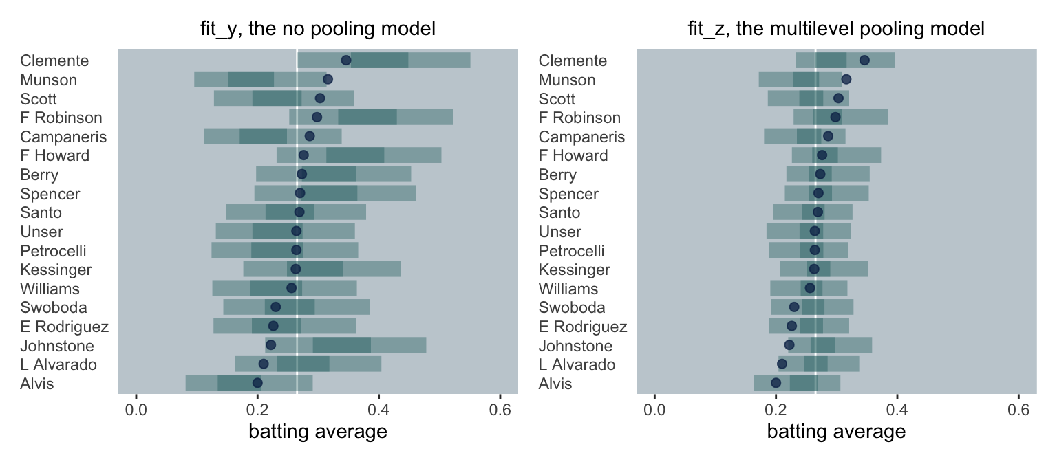
In both panels, the end-of-the-season batting averages (i.e., \(\theta\)) are the blue dots. The model-implied estimates are depicted by 95% and 50% interval bands (i.e., the lighter and darker green horizontal lines, respectively). The white line in the background marks off the mean of \(\theta\). Although neither model was perfect, the multilevel model, our analogue to the James-Stein estimates, yielded predictions that appear both more valid and more precise.
We might also compare the models by their prediction errors. Here we’ll subtract the end-of-the-season batting averages from the model estimates. But unlike with y and z estimates, above, our fit_y and fit_z models yielded entire posterior distributions. Therefore, we’ll express our prediction errors in terms of error distributions, rather than single values.
# save the `fit_y` plot
p3 <-
  f_y %>%
  # the error distribution is just the model-implied values minus
  # the true end-of-season values
  mutate(error = mu - true_ba)  %>%
  ggplot(aes(x = error, y = reorder(player, true_ba))) +
  geom_vline(xintercept = c(0, -.2, .2), size = c(1/2, 1/4, 1/4),
             linetype = c(1, 3, 3), color = "white") +
  stat_halfeye(point_interval = mean_qi, .width = .95,
               color = navy_blue, fill = alpha(nw_green, 2/3)) +
  coord_cartesian(xlim = c(-.35, .35)) +
  labs(subtitle = "fit_y, the no pooling model",
       x = "error",
       y = NULL) +
  theme(axis.text.y = element_text(hjust = 0),
        axis.ticks.y = element_blank(),
        plot.subtitle = element_text(hjust = .5))
# save the `fit_z` plot
p4 <-
  f_z %>%
  mutate(error = mu - true_ba)  %>%

  ggplot(aes(x = error, y = reorder(player, true_ba))) +
  geom_vline(xintercept = c(0, -.2, .2), size = c(1/2, 1/4, 1/4),
             linetype = c(1, 3, 3), color = "white") +
  stat_halfeye(point_interval = mean_qi, .width = .95,
               color = navy_blue, fill = alpha(nw_green, 2/3)) +
  coord_cartesian(xlim = c(-.35, .35)) +
  labs(subtitle = "fit_z, the multilevel pooling model",
       x = "error",
       y = NULL) +
  theme(axis.text.y = element_text(hjust = 0),
        axis.ticks.y = element_blank(),
        plot.subtitle = element_text(hjust = .5))
# now combine the two and behold
p3 | p4
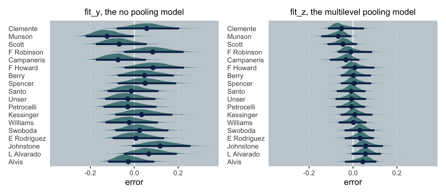
For consistency, I’ve ordered the players along the \(y\)-axis the same as above. In both panels, we see the prediction error distribution for each player in green and then summarize those distributions in terms of their means and percentile-based 95% intervals. Since these are error distributions, we prefer them to be as close to zero as possible. Although neither model made perfect predictions, the overall errors in the multilevel model were clearly smaller. Much like with the James-Stein estimator, the partial pooling of the multilevel model made for better end-of-the-season estimates.
The paradoxical [consequence of Bayesian multilevel models] is that [they can contradict] this elementary law of statistical theory. If we have [two] or more baseball players, and if we are interested in predicting future batting averages for each of them, then [the Bayesian multilevel model can be better] than simply extrapolating from [the] separate averages. ( Efron & Morris, 1977.), p. 119] This is another example of how the KISS principle isn’t always the best bet with data analysis.
Next steps
If you’re new to logistic regression, multilevel models or Bayesian statistics, I recommend any of the following texts:
- either edition of McElreath’s ( 2020, 2015) Statistical rethinking, both editions for which I have brms translations for ( Kurz, 2020b, 2020c);
- Kruschke’s ( 2015) Doing Bayesian data analysis, for which I have a brms translation ( Kurz, 2020a); or
- Gelman and Hill’s ( 2006) Data analysis using regression and multilevel/hierarchical models.
If you choose Statistical rethinking, do check out these great lectures on the text.
Also, don’t miss the provocative ( 2017) preprint by Davis-Stober, Dana and Rouder, When are sample means meaningful? The role of modern estimation in psychological science.
Session info
sessionInfo()
## R version 4.2.0 (2022-04-22)
## Platform: x86_64-apple-darwin17.0 (64-bit)
## Running under: macOS Big Sur/Monterey 10.16
##
## Matrix products: default
## BLAS:   /Library/Frameworks/R.framework/Versions/4.2/Resources/lib/libRblas.0.dylib
## LAPACK: /Library/Frameworks/R.framework/Versions/4.2/Resources/lib/libRlapack.dylib
##
## locale:
## [1] en_US.UTF-8/en_US.UTF-8/en_US.UTF-8/C/en_US.UTF-8/en_US.UTF-8
##
## attached base packages:
## [1] stats     graphics  grDevices utils     datasets  methods   base
##
## other attached packages:
##  [1] patchwork_1.1.2 brms_2.18.0     Rcpp_1.0.9      tidybayes_3.0.2 forcats_0.5.1   stringr_1.4.1
##  [7] dplyr_1.0.10    purrr_0.3.4     readr_2.1.2     tidyr_1.2.1     tibble_3.1.8    ggplot2_3.4.0
## [13] tidyverse_1.3.2
##
## loaded via a namespace (and not attached):
##   [1] readxl_1.4.1         backports_1.4.1      plyr_1.8.7           igraph_1.3.4
##   [5] svUnit_1.0.6         splines_4.2.0        crosstalk_1.2.0      TH.data_1.1-1
##   [9] rstantools_2.2.0     inline_0.3.19        digest_0.6.30        htmltools_0.5.3
##  [13] fansi_1.0.3          magrittr_2.0.3       checkmate_2.1.0      googlesheets4_1.0.1
##  [17] tzdb_0.3.0           modelr_0.1.8         RcppParallel_5.1.5   matrixStats_0.62.0
##  [21] xts_0.12.1           sandwich_3.0-2       prettyunits_1.1.1    colorspace_2.0-3
##  [25] rvest_1.0.2          ggdist_3.2.0         haven_2.5.1          xfun_0.35
##  [29] callr_3.7.3          crayon_1.5.2         jsonlite_1.8.3       lme4_1.1-31
##  [33] survival_3.4-0       zoo_1.8-10           glue_1.6.2           gtable_0.3.1
##  [37] gargle_1.2.0         emmeans_1.8.0        distributional_0.3.1 pkgbuild_1.3.1
##  [41] rstan_2.21.7         abind_1.4-5          scales_1.2.1         mvtnorm_1.1-3
##  [45] DBI_1.1.3            miniUI_0.1.1.1       viridisLite_0.4.1    xtable_1.8-4
##  [49] stats4_4.2.0         StanHeaders_2.21.0-7 DT_0.24              htmlwidgets_1.5.4
##  [53] httr_1.4.4           threejs_0.3.3        arrayhelpers_1.1-0   posterior_1.3.1
##  [57] ellipsis_0.3.2       pkgconfig_2.0.3      loo_2.5.1            farver_2.1.1
##  [61] sass_0.4.2           dbplyr_2.2.1         utf8_1.2.2           labeling_0.4.2
##  [65] tidyselect_1.1.2     rlang_1.0.6          reshape2_1.4.4       later_1.3.0
##  [69] munsell_0.5.0        cellranger_1.1.0     tools_4.2.0          cachem_1.0.6
##  [73] cli_3.4.1            generics_0.1.3       broom_1.0.1          ggridges_0.5.3
##  [77] evaluate_0.18        fastmap_1.1.0        yaml_2.3.5           processx_3.8.0
##  [81] knitr_1.40           fs_1.5.2             nlme_3.1-159         mime_0.12
##  [85] projpred_2.2.1       xml2_1.3.3           compiler_4.2.0       bayesplot_1.9.0
##  [89] shinythemes_1.2.0    rstudioapi_0.13      gamm4_0.2-6          reprex_2.0.2
##  [93] bslib_0.4.0          stringi_1.7.8        highr_0.9            ps_1.7.2
##  [97] blogdown_1.15        Brobdingnag_1.2-8    lattice_0.20-45      Matrix_1.4-1
## [101] nloptr_2.0.3         markdown_1.1         shinyjs_2.1.0        tensorA_0.36.2
## [105] vctrs_0.5.0          pillar_1.8.1         lifecycle_1.0.3      jquerylib_0.1.4
## [109] bridgesampling_1.1-2 estimability_1.4.1   httpuv_1.6.5         R6_2.5.1
## [113] bookdown_0.28        promises_1.2.0.1     gridExtra_2.3        codetools_0.2-18
## [117] boot_1.3-28          colourpicker_1.1.1   MASS_7.3-58.1        gtools_3.9.3
## [121] assertthat_0.2.1     withr_2.5.0          shinystan_2.6.0      multcomp_1.4-20
## [125] mgcv_1.8-40          parallel_4.2.0       hms_1.1.1            grid_4.2.0
## [129] coda_0.19-4          minqa_1.2.5          rmarkdown_2.16       googledrive_2.0.0
## [133] shiny_1.7.2          lubridate_1.8.0      base64enc_0.1-3      dygraphs_1.1.1.6
References
Bürkner, P.-C. (2017). brms: An R package for Bayesian multilevel models using Stan. Journal of Statistical Software, 80(1), 1–28. https://doi.org/10.18637/jss.v080.i01
Bürkner, P.-C. (2018). Advanced Bayesian multilevel modeling with the R package brms. The R Journal, 10(1), 395–411. https://doi.org/10.32614/RJ-2018-017
Bürkner, P.-C. (2022). brms: Bayesian regression models using ’Stan’. https://CRAN.R-project.org/package=brms
Davis-Stober, C., Dana, J., & Rouder, J. (2017). When are sample means meaningful? The role of modern estimation in psychological science. OSF Preprints. https://doi.org/10.31219/osf.io/2ukxj
Efron, B. (2010). Empirical Bayes and the James-Stein estimator. In Large-scale inference: Empirical Bayes methods for estimation, testing, and prediction. Cambridge University Press. https://statweb.stanford.edu/~ckirby/brad/LSI/monograph_CUP.pdf
Efron, B., & Morris, C. (1977). Stein’s paradox in statistics. Scientific American, 236(5), 119–127. https://doi.org/10.1038/scientificamerican0577-119
Gelman, A., & Hill, J. (2006). Data analysis using regression and multilevel/hierarchical models. Cambridge University Press. https://doi.org/10.1017/CBO9780511790942
Kay, M. (2022). tidybayes: Tidy data and ’geoms’ for Bayesian models. https://CRAN.R-project.org/package=tidybayes
Kruschke, J. K. (2015). Doing Bayesian data analysis: A tutorial with R, JAGS, and Stan. Academic Press. https://sites.google.com/site/doingbayesiandataanalysis/
Kurz, A. S. (2020a). Doing Bayesian data analysis in brms and the tidyverse (version 0.3.0). https://bookdown.org/content/3686/
Kurz, A. S. (2020b). Statistical rethinking with brms, Ggplot2, and the tidyverse: Second edition (version 0.1.1). https://bookdown.org/content/4857/
Kurz, A. S. (2020c). Statistical rethinking with brms, ggplot2, and the tidyverse (version 1.2.0). https://doi.org/10.5281/zenodo.3693202
McElreath, R. (2020). Statistical rethinking: A Bayesian course with examples in R and Stan (Second Edition). CRC Press. https://xcelab.net/rm/statistical-rethinking/
McElreath, R. (2015). Statistical rethinking: A Bayesian course with examples in R and Stan. CRC press. https://xcelab.net/rm/statistical-rethinking/
Pedersen, T. L. (2022). patchwork: The composer of plots. https://CRAN.R-project.org/package=patchwork
R Core Team. (2022). R: A language and environment for statistical computing. R Foundation for Statistical Computing. https://www.R-project.org/
Wickham, H. (2022). tidyverse: Easily install and load the ’tidyverse’. https://CRAN.R-project.org/package=tidyverse
Wickham, H., Averick, M., Bryan, J., Chang, W., McGowan, L. D., François, R., Grolemund, G., Hayes, A., Henry, L., Hester, J., Kuhn, M., Pedersen, T. L., Miller, E., Bache, S. M., Müller, K., Ooms, J., Robinson, D., Seidel, D. P., Spinu, V., … Yutani, H. (2019). Welcome to the tidyverse. Journal of Open Source Software, 4(43), 1686. https://doi.org/10.21105/joss.01686
- Posted on:
- February 23, 2019
- Length:
- 26 minute read, 5359 words
- Tags:
- Bayesian brms multilevel R tutorial