Bayesian Correlations: Let's Talk Options.
By A. Solomon Kurz
February 16, 2019
[edited Dec 11, 2022]
tl;dr
There’s more than one way to fit a Bayesian correlation in brms.
Here’s the deal.
In the last post, we considered how we might estimate correlations when our data contain influential outlier values. Our big insight was that if we use variants of Student’s \(t\)-distribution as the likelihood rather than the conventional normal distribution, our correlation estimates were less influenced by those outliers. And we mainly did that as Bayesians using the
brms package. Click
here for a refresher.
Since the brms package is designed to fit regression models, it can be surprising when you discover it’s handy for correlations, too. In short, you can fit them using a few tricks based on the multivariate syntax.
Shortly after uploading the post, it occurred to me we had more options and it might be useful to walk through them a bit.
I assume things.
For this post, I’m presuming you are vaguely familiar with linear regression–both univariate and multivariate–, have a little background with Bayesian statistics, and have used Paul Bürkner’s brms packge. As you might imagine, all code in is R, with a heavy use of the tidyverse.
We need data.
First, we’ll load our main packages.
library(mvtnorm)
library(brms)
library(tidyverse)
We’ll use the mvtnorm package to simulate three positively correlated variables.
m <- c(10, 15, 20)  # the means
s <- c(10, 20, 30)  # the sigmas
r <- c(.9, .6, .3)  # the correlations

# here's the variance/covariance matrix
v <-
  matrix(c((s[1] * s[1]),        (s[2] * s[1] * r[1]), (s[3] * s[1] * r[2]),
           (s[2] * s[1] * r[1]), (s[2] * s[2]),        (s[3] * s[2] * r[3]),
           (s[3] * s[1] * r[2]), (s[3] * s[2] * r[3]), (s[3] * s[3])),
         nrow = 3, ncol = 3)

# after setting our seed, we're ready to simulate with `rmvnorm()`
set.seed(1)
d <-
  rmvnorm(n = 50, mean = m, sigma = v) %>%
  as_tibble() %>%
  set_names("x", "y", "z")
Our data look like so.
library(GGally)
theme_set(theme_gray() +
            theme(panel.grid = element_blank()))

d %>%
  ggpairs(upper = list(continuous = wrap("cor", stars = FALSE)))
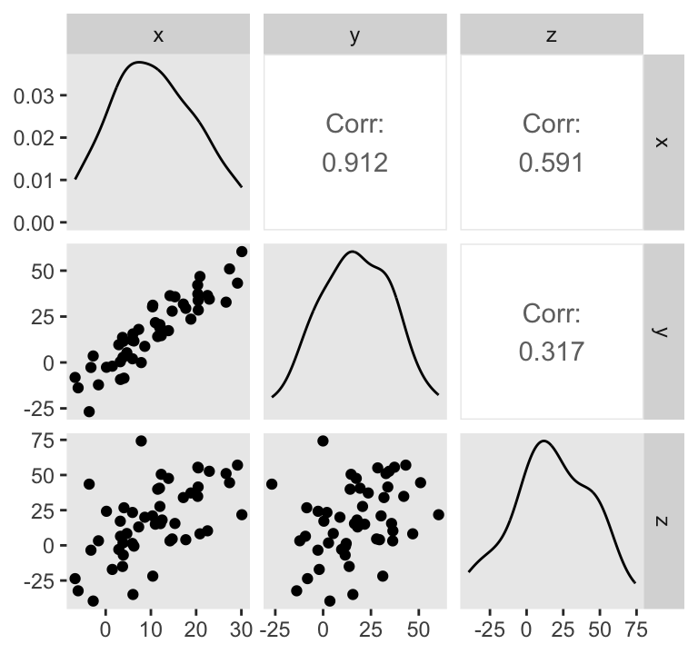
Do note the Pearson’s correlation coefficients in the upper triangle.
In order to exploit all the methods we’ll cover in this post, we need to standardize our data. Here we do so by hand using the typical formula
$$z_{x_i} = \frac{x_i - \overline x}{s_x}$$
where \(\overline x\) is the observed mean and \(s_x\) is the observed standard deviation.
d <-
  d %>%
  mutate(x_s = (x - mean(x)) / sd(x),
         y_s = (y - mean(y)) / sd(y),
         z_s = (z - mean(z)) / sd(z))

head(d)
## # A tibble: 6 × 6
##       x     y     z    x_s      y_s    z_s
##   <dbl> <dbl> <dbl>  <dbl>    <dbl>  <dbl>
## 1  3.90  11.5 -6.90 -0.723 -0.308   -0.928
## 2 17.7   29.5  4.01  0.758  0.653   -0.512
## 3 20.4   33.8 41.5   1.05   0.886    0.917
## 4 20.3   42.1 34.8   1.04   1.33     0.663
## 5 -3.64 -26.8 43.5  -1.53  -2.36     0.994
## 6 13.9   17.3 47.6   0.347  0.00255  1.15
There are at least two broad ways to get correlations out of standardized data in brms. One way uses the typical univariate syntax. The other way is an extension of the multivariate cbind() approach. Let’s start univariate.
And for a point of clarification, we’re presuming the Gaussian likelihood for all the examples in this post.
Univariate
If you fit a simple univariate model with standardized data and a single predictor, the coefficient for the slope will be in a correlation-like metric. Happily, since the data are all standardized, it’s easy to use regularizing priors.
f1 <-
  brm(data = d,
      family = gaussian,
      y_s ~ 1 + x_s,
      prior = c(prior(normal(0, 1), class = Intercept),
                prior(normal(0, 1), class = b),
                prior(normal(0, 1), class = sigma)),
      chains = 4, cores = 4,
      seed = 1)
Take a look at the model summary.
print(f1)
##  Family: gaussian
##   Links: mu = identity; sigma = identity
## Formula: y_s ~ 1 + x_s
##    Data: d (Number of observations: 50)
##   Draws: 4 chains, each with iter = 2000; warmup = 1000; thin = 1;
##          total post-warmup draws = 4000
##
## Population-Level Effects:
##           Estimate Est.Error l-95% CI u-95% CI Rhat Bulk_ESS Tail_ESS
## Intercept     0.00      0.06    -0.13     0.12 1.00     3718     2422
## x_s           0.91      0.06     0.79     1.03 1.00     3756     2874
##
## Family Specific Parameters:
##       Estimate Est.Error l-95% CI u-95% CI Rhat Bulk_ESS Tail_ESS
## sigma     0.42      0.04     0.35     0.52 1.00     3209     2812
##
## Draws were sampled using sampling(NUTS). For each parameter, Bulk_ESS
## and Tail_ESS are effective sample size measures, and Rhat is the potential
## scale reduction factor on split chains (at convergence, Rhat = 1).
The ‘Population-Level Effects’ has the summary information for our intercept and slope. Notice how our x_s slope is the same as the Pearson’s correlation.
cor(d$x, d$y)
## [1] 0.9119708
Since this approach only yields one correlation at a time, we have to fit two more models to get the other two correlations. To do so with haste, we can use the update() syntax.
f2 <-
  update(f1,
         newdata = d,
         formula = z_s ~ 1 + x_s)

f3 <-
  update(f2,
         newdata = d,
         formula = z_s ~ 1 + y_s)
With the fixef() function, we can easily isolate the \(\beta\) estimates.
fixef(f2)[2, ]
##  Estimate Est.Error      Q2.5     Q97.5
## 0.5826984 0.1194922 0.3459339 0.8149767
fixef(f3)[2, ]
##   Estimate  Est.Error       Q2.5      Q97.5
## 0.30874774 0.13877552 0.03055009 0.57645259
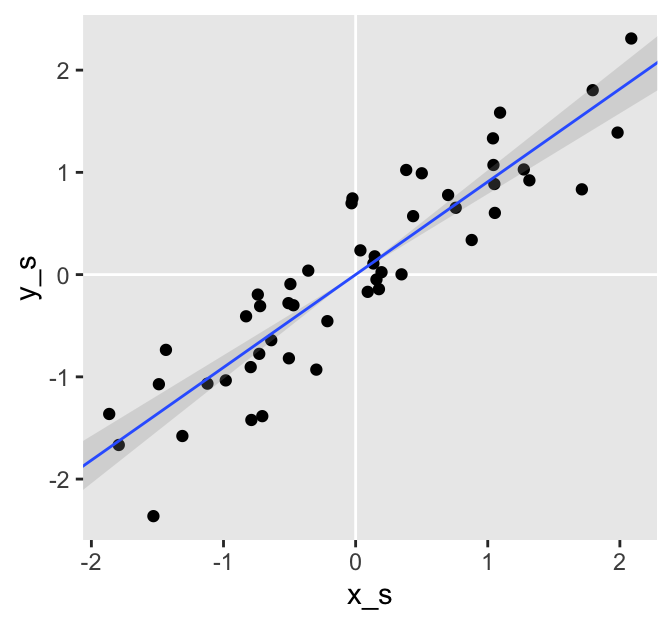
There’s another thing I’d like to point out. Plotting the model results will help make the point.
# define the predictor values you'd like the fitted values for
nd <- tibble(x_s = seq(from = -3, to = 3, length.out = d %>% nrow()))

# wrangle
fitted(f1,
       newdata = nd) %>%
  data.frame() %>%
  bind_cols(nd) %>%

  # plot
  ggplot(aes(x_s)) +
  geom_vline(xintercept = 0, color = "white") +
  geom_hline(yintercept = 0, color = "white") +
  geom_point(data = d,
             aes(y = y_s)) +
  geom_smooth(aes(y = Estimate, ymin = Q2.5, ymax = Q97.5),
              stat = "identity",
              alpha = 1/4, size = 1/2) +
  coord_cartesian(xlim = range(d$x_s),
                  ylim = range(d$y_s))
## Warning: Using `size` aesthetic for lines was deprecated in ggplot2 3.4.0.
## ℹ Please use `linewidth` instead.

The blue line is the posterior mean and the surrounding gray ribbon depicts the 95% posterior interval. Notice how the data and their respective fitted lines pass through [0, 0]? This is a consequence of modeling standardized data. We should always expect the intercept of a model like this to be 0. Here are the intercept summaries for all three models.
fixef(f1)["Intercept", ] %>% round(3)
##  Estimate Est.Error      Q2.5     Q97.5
##     0.001     0.062    -0.126     0.118
fixef(f2)["Intercept", ] %>% round(3)
##  Estimate Est.Error      Q2.5     Q97.5
##    -0.001     0.119    -0.234     0.234
fixef(f3)["Intercept", ] %>% round(3)
##  Estimate Est.Error      Q2.5     Q97.5
##    -0.001     0.137    -0.271     0.269
Within simulation error, they’re all centered on zero. So instead of estimating the intercept, why not just bake that into the models? Here we refit the models by fixing the intercept for each to zero.
f4 <-
  update(f1,
         formula = y_s ~ 0 + x_s)

f5 <-
  update(f4,
         newdata = d,
         formula = z_s ~ 0 + x_s)

f6 <-
  update(f4,
         newdata = d,
         formula = z_s ~ 0 + y_s)
Let’s take a look at the summary for the first.
print(f4)
##  Family: gaussian
##   Links: mu = identity; sigma = identity
## Formula: y_s ~ x_s - 1
##    Data: d (Number of observations: 50)
##   Draws: 4 chains, each with iter = 2000; warmup = 1000; thin = 1;
##          total post-warmup draws = 4000
##
## Population-Level Effects:
##     Estimate Est.Error l-95% CI u-95% CI Rhat Bulk_ESS Tail_ESS
## x_s     0.91      0.06     0.79     1.02 1.00     3286     2475
##
## Family Specific Parameters:
##       Estimate Est.Error l-95% CI u-95% CI Rhat Bulk_ESS Tail_ESS
## sigma     0.42      0.04     0.34     0.52 1.00     3499     2542
##
## Draws were sampled using sampling(NUTS). For each parameter, Bulk_ESS
## and Tail_ESS are effective sample size measures, and Rhat is the potential
## scale reduction factor on split chains (at convergence, Rhat = 1).
Even though it may have seemed like we substantially changed the models by fixing the intercepts to 0, the summaries are essentially the same as when we estimated the intercepts. Here we’ll confirm the summaries with a plot, like above.
# wrangle
fitted(f4,
       newdata = nd) %>%
  data.frame() %>%
  bind_cols(nd) %>%

  # plot
  ggplot(aes(x_s)) +
  geom_vline(xintercept = 0, color = "white") +
  geom_hline(yintercept = 0, color = "white") +
  geom_point(data = d,
             aes(y = y_s)) +
  geom_smooth(aes(y = Estimate, ymin = Q2.5, ymax = Q97.5),
              stat = "identity",
              alpha = 1/4, size = 1/2) +
  coord_cartesian(xlim = range(d$x_s),
                  ylim = range(d$y_s))
The difference is subtle. By fixing the intercepts at 0, we estimated the slopes (i.e., the correlations) with increased precision as demonstrated by the slightly smaller posterior standard deviations (i.e., the values in the ‘Est.Error’ columns).
Here are the correlation summaries for those last three models.
fixef(f4) %>% round(3)
##     Estimate Est.Error  Q2.5 Q97.5
## x_s    0.908     0.059 0.789 1.021
fixef(f5) %>% round(3)
##     Estimate Est.Error  Q2.5 Q97.5
## x_s    0.579     0.118 0.341 0.808
fixef(f6) %>% round(3)
##     Estimate Est.Error  Q2.5 Q97.5
## y_s    0.312     0.141 0.044 0.597
But anyway, you get the idea. If you want to estimate a correlation in brms using simple univariate syntax, just (a) standardize the data and (b) fit a univariate model with or without an intercept. The slop will be in a correlation-like metric.
Let’s go multivariate.
If you don’t recall the steps to fit correlations in brms with the multivariate syntax, here they are:
- List the variables you’d like correlations for within
mvbind(). - Place the
mvbind()function within the left side of the model formula. - On the right side of the model formula, indicate you only want intercepts (i.e.,
~ 1). - Wrap that whole formula within
bf(). - Then use the
+operator to appendset_rescor(TRUE), which will ensure brms fits a model with residual correlations.
In addition, you you want to use non-default priors, you’ll want to use the resp argument to specify which prior is associated with which criterion variable. Here’s what that all looks like:
f7 <-
  brm(data = d,
      family = gaussian,
      bf(mvbind(x_s, y_s, z_s) ~ 1) + set_rescor(TRUE),
      prior = c(prior(normal(0, 1), class = Intercept, resp = xs),
                prior(normal(0, 1), class = Intercept, resp = ys),
                prior(normal(0, 1), class = Intercept, resp = zs),
                prior(normal(1, 1), class = sigma, resp = xs),
                prior(normal(1, 1), class = sigma, resp = ys),
                prior(normal(1, 1), class = sigma, resp = zs),
                prior(lkj(2), class = rescor)),
      chains = 4, cores = 4,
      seed = 1)
Behold the summary.
print(f7)
##  Family: MV(gaussian, gaussian, gaussian)
##   Links: mu = identity; sigma = identity
##          mu = identity; sigma = identity
##          mu = identity; sigma = identity
## Formula: x_s ~ 1
##          y_s ~ 1
##          z_s ~ 1
##    Data: d (Number of observations: 50)
##   Draws: 4 chains, each with iter = 2000; warmup = 1000; thin = 1;
##          total post-warmup draws = 4000
##
## Population-Level Effects:
##              Estimate Est.Error l-95% CI u-95% CI Rhat Bulk_ESS Tail_ESS
## xs_Intercept    -0.00      0.13    -0.26     0.26 1.00     2026     2269
## ys_Intercept    -0.00      0.14    -0.27     0.27 1.00     2292     2784
## zs_Intercept    -0.00      0.14    -0.28     0.27 1.00     2966     2695
##
## Family Specific Parameters:
##          Estimate Est.Error l-95% CI u-95% CI Rhat Bulk_ESS Tail_ESS
## sigma_xs     0.99      0.10     0.82     1.20 1.00     1730     2325
## sigma_ys     1.00      0.10     0.82     1.22 1.00     1722     2815
## sigma_zs     1.03      0.11     0.85     1.26 1.00     3260     2682
##
## Residual Correlations:
##               Estimate Est.Error l-95% CI u-95% CI Rhat Bulk_ESS Tail_ESS
## rescor(xs,ys)     0.89      0.03     0.83     0.94 1.00     2099     2480
## rescor(xs,zs)     0.55      0.10     0.34     0.72 1.00     3089     2798
## rescor(ys,zs)     0.25      0.13    -0.02     0.49 1.00     2781     2438
##
## Draws were sampled using sampling(NUTS). For each parameter, Bulk_ESS
## and Tail_ESS are effective sample size measures, and Rhat is the potential
## scale reduction factor on split chains (at convergence, Rhat = 1).
Look at the ‘Residual Correlations:’ section at the bottom of the output. Since there are no predictors in the model, the residual correlations are just correlations. Now notice how the intercepts in this model are also hovering around 0, just like in our univariate models. Yep, we can fix those, too. We do this by changing our formula to mvbind(x_s, y_s, z_s) ~ 0.
f8 <-
  brm(data = d,
      family = gaussian,
      bf(mvbind(x_s, y_s, z_s) ~ 0) + set_rescor(TRUE),
      prior = c(prior(normal(1, 1), class = sigma, resp = xs),
                prior(normal(1, 1), class = sigma, resp = ys),
                prior(normal(1, 1), class = sigma, resp = zs),
                prior(lkj(2), class = rescor)),
      chains = 4, cores = 4,
      seed = 1)
Without the intercepts, the rest of the model is the same within simulation variance.
print(f8)
##  Family: MV(gaussian, gaussian, gaussian)
##   Links: mu = identity; sigma = identity
##          mu = identity; sigma = identity
##          mu = identity; sigma = identity
## Formula: x_s ~ 0
##          y_s ~ 0
##          z_s ~ 0
##    Data: d (Number of observations: 50)
##   Draws: 4 chains, each with iter = 2000; warmup = 1000; thin = 1;
##          total post-warmup draws = 4000
##
## Family Specific Parameters:
##          Estimate Est.Error l-95% CI u-95% CI Rhat Bulk_ESS Tail_ESS
## sigma_xs     0.98      0.09     0.81     1.19 1.00     1734     2118
## sigma_ys     0.99      0.10     0.83     1.21 1.00     1900     2102
## sigma_zs     1.02      0.11     0.83     1.25 1.00     2467     2189
##
## Residual Correlations:
##               Estimate Est.Error l-95% CI u-95% CI Rhat Bulk_ESS Tail_ESS
## rescor(xs,ys)     0.90      0.03     0.83     0.94 1.00     2026     2350
## rescor(xs,zs)     0.55      0.09     0.35     0.72 1.00     2935     2670
## rescor(ys,zs)     0.26      0.13     0.00     0.49 1.00     2509     2408
##
## Draws were sampled using sampling(NUTS). For each parameter, Bulk_ESS
## and Tail_ESS are effective sample size measures, and Rhat is the potential
## scale reduction factor on split chains (at convergence, Rhat = 1).
If you wanna get silly, we can prune even further. Did you notice how the estimates for \(\sigma\) are all hovering around 1? Since we have no predictors, \(\sigma\) is just an estimate of the population standard deviation. And since we’re working with standardized data, the population standard deviation has to be 1. Any other estimate would be nonsensical. So why not fix it to 1?
With brms, we can fix those \(\sigma\)’s to 1 with a trick of the nonlinear
distributional modeling syntax. Recall when you model \(\sigma\), the brms default is to actually model its log. As is turns out, the log of 1 is zero.
log(1)
## [1] 0
Here’s how to make use of that within brm().
f9 <-
  brm(data = d,
      family = gaussian,
      bf(mvbind(x_s, y_s, z_s) ~ 0,
         sigma ~ 0) +
        set_rescor(TRUE),
      prior(lkj(2), class = rescor),
      chains = 4, cores = 4,
      seed = 1)
Here are the results.
print(f9)
##  Family: MV(gaussian, gaussian, gaussian)
##   Links: mu = identity; sigma = log
##          mu = identity; sigma = log
##          mu = identity; sigma = log
## Formula: x_s ~ 0
##          sigma ~ 0
##          y_s ~ 0
##          sigma ~ 0
##          z_s ~ 0
##          sigma ~ 0
##    Data: d (Number of observations: 50)
##   Draws: 4 chains, each with iter = 2000; warmup = 1000; thin = 1;
##          total post-warmup draws = 4000
##
## Residual Correlations:
##               Estimate Est.Error l-95% CI u-95% CI Rhat Bulk_ESS Tail_ESS
## rescor(xs,ys)     0.90      0.02     0.86     0.93 1.00     3003     2877
## rescor(xs,zs)     0.57      0.07     0.43     0.69 1.00     3543     3011
## rescor(ys,zs)     0.29      0.09     0.12     0.46 1.00     2950     2869
##
## Draws were sampled using sampling(NUTS). For each parameter, Bulk_ESS
## and Tail_ESS are effective sample size measures, and Rhat is the potential
## scale reduction factor on split chains (at convergence, Rhat = 1).
The correlations are the only things left in the model.
Just to be clear, the multivariate approach does not require standardized data. To demonstrate, here we refit f7, but with the unstandardized variables. And, since we’re no longer in the standardized metric, we’ll be less certain with our priors.
f10 <-
  brm(data = d,
      family = gaussian,
      bf(mvbind(x, y, z) ~ 1) + set_rescor(TRUE),
      prior = c(prior(normal(0, 10), class = Intercept, resp = x),
                prior(normal(0, 10), class = Intercept, resp = y),
                prior(normal(0, 10), class = Intercept, resp = z),
                prior(student_t(3, 0, 10), class = sigma, resp = x),
                prior(student_t(3, 0, 10), class = sigma, resp = y),
                prior(student_t(3, 0, 10), class = sigma, resp = z),
                prior(lkj(2), class = rescor)),
      chains = 4, cores = 4,
      seed = 1)
See, the ‘rescor()’ results are about the same as with f7.
print(f10)
##  Family: MV(gaussian, gaussian, gaussian)
##   Links: mu = identity; sigma = identity
##          mu = identity; sigma = identity
##          mu = identity; sigma = identity
## Formula: x ~ 1
##          y ~ 1
##          z ~ 1
##    Data: d (Number of observations: 50)
##   Draws: 4 chains, each with iter = 2000; warmup = 1000; thin = 1;
##          total post-warmup draws = 4000
##
## Population-Level Effects:
##             Estimate Est.Error l-95% CI u-95% CI Rhat Bulk_ESS Tail_ESS
## x_Intercept     9.65      1.22     7.18    11.99 1.00     2020     2106
## y_Intercept    15.62      2.49    10.69    20.41 1.00     2194     2113
## z_Intercept    14.77      3.47     7.79    21.35 1.00     3070     2977
##
## Family Specific Parameters:
##         Estimate Est.Error l-95% CI u-95% CI Rhat Bulk_ESS Tail_ESS
## sigma_x     8.98      0.87     7.47    10.92 1.00     2054     2469
## sigma_y    18.17      1.80    15.08    22.19 1.00     2401     2259
## sigma_z    26.17      2.56    21.77    31.70 1.00     3001     2697
##
## Residual Correlations:
##             Estimate Est.Error l-95% CI u-95% CI Rhat Bulk_ESS Tail_ESS
## rescor(x,y)     0.89      0.03     0.82     0.94 1.00     2212     2539
## rescor(x,z)     0.55      0.09     0.36     0.71 1.00     2935     2613
## rescor(y,z)     0.25      0.12     0.01     0.48 1.00     2625     2736
##
## Draws were sampled using sampling(NUTS). For each parameter, Bulk_ESS
## and Tail_ESS are effective sample size measures, and Rhat is the potential
## scale reduction factor on split chains (at convergence, Rhat = 1).
It’s time to compare methods.
To recap, we’ve compared several ways to fit correlations in brms. Some of the methods were with univariate syntax, others were with the multivariate syntax. Some of the models had all free parameters, others included fixed intercepts and sigmas. Whereas all the univariate models required standardized data, the multivariate approach can work with unstandardized data, too.
Now it might be of help to compare the results from each of the methods to get a sense of which ones you might prefer. Before we do so, we’ll define a couple custom functions to streamline the data wrangling.
get_rho <- function(fit) {
  as_draws_df(fit) %>%
    select(starts_with("b_"), -contains("Intercept")) %>%
    set_names("rho")
}

get_rescor <- function(fit) {
  as_draws_df(fit) %>%
    select(starts_with("rescor")) %>%
    set_names("x with y", "x with z", "y with z") %>%
    gather(label, rho) %>%
    select(rho, label)
}
Now let’s put those functions to work and plot.
library(tidybayes)

# collect the posteriors from the univariate models
tibble(name = str_c("f", 1:6)) %>%
  mutate(fit = map(name, get)) %>%
  mutate(rho = map(fit, get_rho)) %>%
  unnest(rho) %>%
  mutate(predictor = rep(c("x", "x", "y"), each = 4000) %>% rep(., times = 2),
         criterion = rep(c("y", "z", "z"), each = 4000) %>% rep(., times = 2)) %>%
  mutate(label = str_c(predictor, " with ", criterion)) %>%
  select(-c(predictor:criterion)) %>%
  # add in the posteriors from the multivariate models
  bind_rows(
    tibble(name = str_c("f", 7:10)) %>%
      mutate(fit = map(name, get)) %>%
      mutate(post = map(fit, get_rescor)) %>%
      unnest(post)
  ) %>%
  # wrangle a bit just to make the y axis easier to understand
  mutate(name = factor(name,
                       levels = c(str_c("f", 1:10)),
                       labels = c("1. standardized, univariate",
                                  "2. standardized, univariate",
                                  "3. standardized, univariate",
                                  "4. standardized, univariate, fixed intercepts",
                                  "5. standardized, univariate, fixed intercepts",
                                  "6. standardized, univariate, fixed intercepts",
                                  "7. standardized, multivariate, fixed intercepts",
                                  "8. standardized, multivariate, fixed intercepts",
                                  "9. standardized, multivariate, fixed intercepts/sigmas",
                                  "10. unstandardized, multivariate"))) %>%

  # plot
  ggplot(aes(x = rho, y = name)) +
  geom_vline(data = tibble(label = c("x with y", "x with z", "y with z"),
                           rho   = r),
             aes(xintercept = rho), color = "white") +
  stat_halfeye(.width = .95, size = 5/4) +
  scale_x_continuous(breaks = c(0, r)) +
  labs(x = expression(rho),
       y = NULL) +
  coord_cartesian(0:1) +
  theme(axis.ticks.y = element_blank(),
        axis.text.y  = element_text(hjust = 0)) +
  facet_wrap(~ label, ncol = 3)
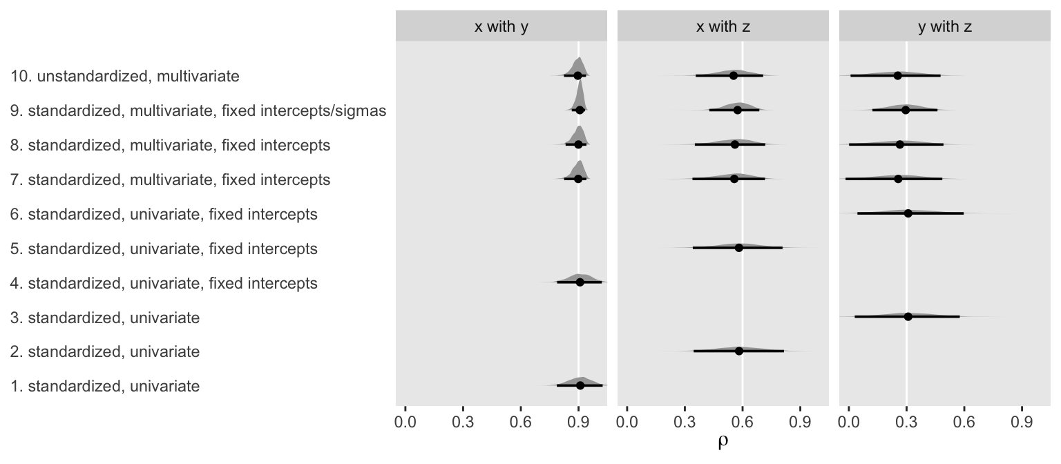
To my eye, a few patterns emerged. First, the point estimates were about the same across methods. Second, fixing the intercepts didn’t seem to effect things, much. But, third, it appears that fixing the sigmas in the multivariate models did narrow the posteriors a bit.
Fourth, and perhaps most importantly, notice how the posteriors for the multivariate models were more asymmetric when they approached 1. Hopefully this makes intuitive sense. Correlations are bound between -1 and 1. However, standardized regression coefficients are not so bound. Accordingly, notice how the posteriors from the univariate models stayed symmetric when approaching 1 and some of their right tails even crossed over 1. So while the univariate approach did a reasonable job capturing the correlation point estimates, their posteriors weren’t quite in a correlation metric. Alternately, the univariate approach did make it convenient to express the correlations with fitted regression lines in scatter plots.
Both univariate and multivariate approaches appear to have their strengths and weaknesses. Choose which methods seems most appropriate for your correlation needs.
Happy modeling.
sessionInfo()
## R version 4.2.0 (2022-04-22)
## Platform: x86_64-apple-darwin17.0 (64-bit)
## Running under: macOS Big Sur/Monterey 10.16
##
## Matrix products: default
## BLAS:   /Library/Frameworks/R.framework/Versions/4.2/Resources/lib/libRblas.0.dylib
## LAPACK: /Library/Frameworks/R.framework/Versions/4.2/Resources/lib/libRlapack.dylib
##
## locale:
## [1] en_US.UTF-8/en_US.UTF-8/en_US.UTF-8/C/en_US.UTF-8/en_US.UTF-8
##
## attached base packages:
## [1] stats     graphics  grDevices utils     datasets  methods   base
##
## other attached packages:
##  [1] tidybayes_3.0.2 GGally_2.1.2    forcats_0.5.1   stringr_1.4.1
##  [5] dplyr_1.0.10    purrr_0.3.4     readr_2.1.2     tidyr_1.2.1
##  [9] tibble_3.1.8    ggplot2_3.4.0   tidyverse_1.3.2 brms_2.18.0
## [13] Rcpp_1.0.9      mvtnorm_1.1-3
##
## loaded via a namespace (and not attached):
##   [1] readxl_1.4.1         backports_1.4.1      plyr_1.8.7
##   [4] igraph_1.3.4         svUnit_1.0.6         splines_4.2.0
##   [7] crosstalk_1.2.0      TH.data_1.1-1        rstantools_2.2.0
##  [10] inline_0.3.19        digest_0.6.30        htmltools_0.5.3
##  [13] fansi_1.0.3          magrittr_2.0.3       checkmate_2.1.0
##  [16] googlesheets4_1.0.1  tzdb_0.3.0           modelr_0.1.8
##  [19] RcppParallel_5.1.5   matrixStats_0.62.0   xts_0.12.1
##  [22] sandwich_3.0-2       prettyunits_1.1.1    colorspace_2.0-3
##  [25] rvest_1.0.2          ggdist_3.2.0         haven_2.5.1
##  [28] xfun_0.35            callr_3.7.3          crayon_1.5.2
##  [31] jsonlite_1.8.3       lme4_1.1-31          survival_3.4-0
##  [34] zoo_1.8-10           glue_1.6.2           gtable_0.3.1
##  [37] gargle_1.2.0         emmeans_1.8.0        distributional_0.3.1
##  [40] pkgbuild_1.3.1       rstan_2.21.7         abind_1.4-5
##  [43] scales_1.2.1         DBI_1.1.3            miniUI_0.1.1.1
##  [46] xtable_1.8-4         stats4_4.2.0         StanHeaders_2.21.0-7
##  [49] DT_0.24              htmlwidgets_1.5.4    httr_1.4.4
##  [52] threejs_0.3.3        arrayhelpers_1.1-0   RColorBrewer_1.1-3
##  [55] posterior_1.3.1      ellipsis_0.3.2       reshape_0.8.9
##  [58] pkgconfig_2.0.3      loo_2.5.1            farver_2.1.1
##  [61] sass_0.4.2           dbplyr_2.2.1         utf8_1.2.2
##  [64] labeling_0.4.2       tidyselect_1.1.2     rlang_1.0.6
##  [67] reshape2_1.4.4       later_1.3.0          munsell_0.5.0
##  [70] cellranger_1.1.0     tools_4.2.0          cachem_1.0.6
##  [73] cli_3.4.1            generics_0.1.3       broom_1.0.1
##  [76] ggridges_0.5.3       evaluate_0.18        fastmap_1.1.0
##  [79] yaml_2.3.5           processx_3.8.0       knitr_1.40
##  [82] fs_1.5.2             nlme_3.1-159         mime_0.12
##  [85] projpred_2.2.1       xml2_1.3.3           compiler_4.2.0
##  [88] bayesplot_1.9.0      shinythemes_1.2.0    rstudioapi_0.13
##  [91] gamm4_0.2-6          reprex_2.0.2         bslib_0.4.0
##  [94] stringi_1.7.8        highr_0.9            ps_1.7.2
##  [97] blogdown_1.15        Brobdingnag_1.2-8    lattice_0.20-45
## [100] Matrix_1.4-1         nloptr_2.0.3         markdown_1.1
## [103] shinyjs_2.1.0        tensorA_0.36.2       vctrs_0.5.0
## [106] pillar_1.8.1         lifecycle_1.0.3      jquerylib_0.1.4
## [109] bridgesampling_1.1-2 estimability_1.4.1   httpuv_1.6.5
## [112] R6_2.5.1             bookdown_0.28        promises_1.2.0.1
## [115] gridExtra_2.3        codetools_0.2-18     boot_1.3-28
## [118] colourpicker_1.1.1   MASS_7.3-58.1        gtools_3.9.3
## [121] assertthat_0.2.1     withr_2.5.0          shinystan_2.6.0
## [124] multcomp_1.4-20      mgcv_1.8-40          parallel_4.2.0
## [127] hms_1.1.1            grid_4.2.0           coda_0.19-4
## [130] minqa_1.2.5          rmarkdown_2.16       googledrive_2.0.0
## [133] shiny_1.7.2          lubridate_1.8.0      base64enc_0.1-3
## [136] dygraphs_1.1.1.6
- Posted on:
- February 16, 2019
- Length:
- 19 minute read, 3848 words
- Tags:
- Bayesian brms correlation R tutorial