Bayesian robust correlations with brms (and why you should love Student's `\(t\)`)
By A. Solomon Kurz
February 10, 2019
[edited Dec 11, 2022]
In this post, we’ll show how Student’s \(t\)-distribution can produce better correlation estimates when your data have outliers. As is often the case, we’ll do so as Bayesians.
This post is a direct consequence of Adrian Baez-Ortega’s great blog, “ Bayesian robust correlation with Stan in R (and why you should use Bayesian methods)”. Baez-Ortega worked out the approach and code for direct use with Stan computational environment. That solution is great because Stan is free, open source, and very flexible. However, Stan’s interface might be prohibitively technical for non-statistician users. Happily, the brms package allows users to access the computational power of Stan through a simpler interface. In this post, we show how to extend Baez-Ortega’s method to brms. To pay respects where they’re due, the synthetic data, priors, and other model settings are largely the same as those Baez-Ortega used in his blog.
I make assumptions
For this post, I’m presuming you are vaguely familiar with linear regression, know about the basic differences between frequentist and Bayesian approaches to fitting models, and have a sense that the issue of outlier values is a pickle worth contending with. All code in is R, with a heavy use of the tidyverse–which you might learn a lot about here, especially chapter 5–, and, of course, Bürkner’s brms.
If you’d like a warmup, consider checking out my related post,
Robust Linear Regression with Student’s \(t\)-Distribution.
What’s the deal?
Pearson’s correlations are designed to quantify the linear relationship between two normally distributed variables. The normal distribution and its multivariate generalization, the multivariate normal distribution, are sensitive to outliers. When you have well-behaved synthetic data, this isn’t an issue. But if you work real-world data, this can be a problem. One can have data for which the vast majority of cases are well-characterized by a nice liner relationship, but have a few odd cases for which that relationship does not hold. And if those odd cases happen to be overly influential–sometimes called leverage points–the resulting Pearson’s correlation coefficient might look off.
Recall that the normal distribution is a special case of Student’s \(t\)-distribution with the \(\nu\) parameter (i.e., nu, degree of freedom) set to infinity. As it turns out, when \(\nu\) is small, Student’s \(t\)-distribution is more robust to multivariate outliers. It’s less influenced by them. I’m not going to cover why in any detail. For that you’ve got
Baez-Ortega’s blog, an even earlier blog from
Rasmus Bååth, and textbook treatments on the topic by
Gelman & Hill (2007, chapter 6) and
Kruschke (2015, chapter 16). Here we’ll get a quick sense of how vulnerable Pearson’s correlations–with their reliance on the Gaussian–are to outliers, we’ll demonstrate how fitting correlations within the Bayesian paradigm using the conventional Gaussian likelihood is similarly vulnerable to distortion, and then see how Student’s \(t\)-distribution can save the day. And importantly, we’ll do the bulk of this with the brms package.
We need data
To start off, we’ll make a multivariate normal simulated data set using the same steps Baez-Ortega’s used.
library(mvtnorm)
library(tidyverse)

sigma <- c(20, 40)  # the variances
rho   <- -.95       # the desired correlation

# here's the variance/covariance matrix
cov.mat <-
  matrix(c(sigma[1] ^ 2,
           sigma[1] * sigma[2] * rho,
           sigma[1] * sigma[2] * rho,
           sigma[2] ^ 2),
         nrow = 2, byrow = T)

# after setting our seed, we're ready to simulate with `rmvnorm()`
set.seed(210191)
x.clean <-
  rmvnorm(n = 40, sigma = cov.mat) %>%
  as_tibble() %>%
  rename(x = V1,
         y = V2)
Here we make our second data set, x.noisy, which is identical to our well-behaved x.clean data, but with the first three cases transformed to outlier values.
x.noisy <- x.clean

x.noisy[1:3,] <-
  matrix(c(-40, -60,
           20, 100,
           40, 40),
         nrow = 3, byrow = T)
Finally, we’ll add an outlier index to the data sets, which will help us with plotting.
x.clean <-
  x.clean %>%
  mutate(outlier = factor(0))

x.noisy <-
  x.noisy %>%
  mutate(outlier = c(rep(1, 3), rep(0, 37)) %>% as.factor(.))
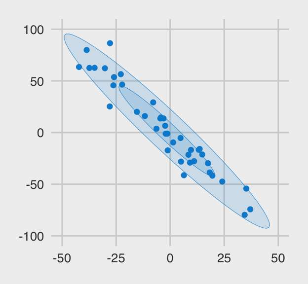
The plot below shows what the x.clean data look like. I’m a fan of
FiveThirtyEight, so we’ll use a few convenience functions from the handy
ggthemes package to give our plots a FiveThirtyEight-like feel.
library(ggthemes)

x.clean %>%
  ggplot(aes(x = x, y = y, color = outlier, fill = outlier)) +
  geom_point() +
  stat_ellipse(geom = "polygon", alpha = .15, size = .15, level = .5) +
  stat_ellipse(geom = "polygon", alpha = .15, size = .15, level = .95) +
  scale_color_fivethirtyeight() +
  scale_fill_fivethirtyeight() +
  coord_cartesian(xlim = c(-50, 50),
                  ylim = c(-100, 100)) +
  theme_fivethirtyeight() +
  theme(legend.position = "none")
And here are the x.noisy data.
x.noisy %>%
  ggplot(aes(x = x, y = y, color = outlier, fill = outlier)) +
  geom_point() +
  stat_ellipse(geom = "polygon", alpha = .15, size = .15, level = .5) +
  stat_ellipse(geom = "polygon", alpha = .15, size = .15, level = .95) +
  scale_color_fivethirtyeight() +
  scale_fill_fivethirtyeight() +
  coord_cartesian(xlim = c(-50, 50),
                  ylim = c(-100, 100)) +
  theme_fivethirtyeight() +
  theme(legend.position = "none")
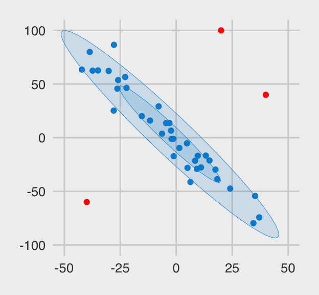
The three outliers are in red. Even in their presence, the old interocular trauma test suggests there is a pronounced overall trend in the data. I would like a correlation procedure that’s capable of capturing that overall trend. Let’s examine some candidates.
How does old Pearson hold up?
A quick way to get a Pearson’s correlation coefficient in R is with the cor() function, which does a nice job recovering the correlation we simulated the x.clean data with:
cor(x.clean$x, x.clean$y)
## [1] -0.959702
However, things fall apart if you use cor() on the x.noisy data.
cor(x.noisy$x, x.noisy$y)
## [1] -0.6365649
So even though most of the x.noisy data continue to show a clear strong relation, three outlier values reduced the Pearson’s correlation a third of the way toward zero. Let’s see what happens when we go Bayesian.
Bayesian correlations in brms
Bürkner’s brms is a general purpose interface for fitting all manner of Bayesian regression models with Stan as the engine under the hood. It has popular lme4-like syntax and offers a variety of convenience functions for post processing. Let’s load it up.
library(brms)
First with the Gaussian likelihood.
I’m not going to spend a lot of time walking through the syntax in the main brms function, brm(). You can learn all about that
here or with my ebook
Statistical Rethinking with brms, ggplot2, and the tidyverse. But our particular use of brm() requires we make a few fine points.
One doesn’t always think about bivariate correlations within the regression paradigm. But they work just fine. Within brms, you would typically specify the conventional Gaussian likelihood (i.e., family = gaussian), use the mvbind() syntax to set up a
multivariate model, and fit that model without predictors. For each variable specified in cbind(), you’ll estimate an intercept (i.e., mean, \(\mu\)) and sigma (i.e., \(\sigma\), often called a residual variance). Since there are no predictors in the model, the residual variance is just the variance and the brms default for multivariate models is to allow the residual variances to covary. But since variances are parameterized in the standard deviation metric in brms, the residual variances and their covariance are SDs and their correlation, respectively.
Here’s what it looks like in practice.
f0 <-
  brm(data = x.clean,
      family = gaussian,
      bf(mvbind(x, y) ~ 1) + set_rescor(TRUE),
      prior = c(prior(normal(0, 100), class = Intercept, resp = x),
                prior(normal(0, 100), class = Intercept, resp = y),
                prior(normal(0, 100), class = sigma, resp = x),
                prior(normal(0, 100), class = sigma, resp = y),
                prior(lkj(1), class = rescor)),
      iter = 2000, warmup = 500, chains = 4, cores = 4,
      seed = 210191)
In a typical Bayesian workflow, you’d examine the quality of the chains with trace plots. The easy way to do that in brms is with plot(). E.g., to get the trace plots for our first model, you’d code plot(f0). Happily, the trace plots look fine for all models in this post. For the sake of space, I’ll leave their inspection as exercises for interested readers.
Our priors and such mirror those in Baez-Ortega’s blog. Here are the results.
print(f0)
##  Family: MV(gaussian, gaussian)
##   Links: mu = identity; sigma = identity
##          mu = identity; sigma = identity
## Formula: x ~ 1
##          y ~ 1
##    Data: x.clean (Number of observations: 40)
##   Draws: 4 chains, each with iter = 2000; warmup = 500; thin = 1;
##          total post-warmup draws = 6000
##
## Population-Level Effects:
##             Estimate Est.Error l-95% CI u-95% CI Rhat Bulk_ESS Tail_ESS
## x_Intercept    -2.88      3.40    -9.56     3.82 1.00     2707     2525
## y_Intercept     3.71      6.80    -9.81    17.15 1.00     2677     2718
##
## Family Specific Parameters:
##         Estimate Est.Error l-95% CI u-95% CI Rhat Bulk_ESS Tail_ESS
## sigma_x    21.52      2.52    17.33    27.02 1.00     1989     2429
## sigma_y    43.05      5.06    34.66    54.28 1.00     1929     2795
##
## Residual Correlations:
##             Estimate Est.Error l-95% CI u-95% CI Rhat Bulk_ESS Tail_ESS
## rescor(x,y)    -0.95      0.02    -0.98    -0.92 1.00     2371     3057
##
## Draws were sampled using sampling(NUTS). For each parameter, Bulk_ESS
## and Tail_ESS are effective sample size measures, and Rhat is the potential
## scale reduction factor on split chains (at convergence, Rhat = 1).
Way down there in the last line in the ‘Family Specific Parameters’ section we have rescor(x,y), which is our correlation. And indeed, our Gaussian intercept-only multivariate model did a great job recovering the correlation we used to simulate the x.clean data with. Look at what happens when we try this approach with x.noisy.
f1 <-
  update(f0,
         newdata = x.noisy,
         iter = 2000, warmup = 500, chains = 4, cores = 4, seed = 210191)
print(f1)
##  Family: MV(gaussian, gaussian)
##   Links: mu = identity; sigma = identity
##          mu = identity; sigma = identity
## Formula: x ~ 1
##          y ~ 1
##    Data: x.noisy (Number of observations: 40)
##   Draws: 4 chains, each with iter = 2000; warmup = 500; thin = 1;
##          total post-warmup draws = 6000
##
## Population-Level Effects:
##             Estimate Est.Error l-95% CI u-95% CI Rhat Bulk_ESS Tail_ESS
## x_Intercept    -3.12      3.78   -10.52     4.29 1.00     4381     4061
## y_Intercept     6.77      7.63    -8.42    21.84 1.00     4590     4071
##
## Family Specific Parameters:
##         Estimate Est.Error l-95% CI u-95% CI Rhat Bulk_ESS Tail_ESS
## sigma_x    23.66      2.78    18.97    29.86 1.00     4415     4377
## sigma_y    47.22      5.45    37.93    58.96 1.00     4562     4354
##
## Residual Correlations:
##             Estimate Est.Error l-95% CI u-95% CI Rhat Bulk_ESS Tail_ESS
## rescor(x,y)    -0.61      0.10    -0.78    -0.38 1.00     4300     4128
##
## Draws were sampled using sampling(NUTS). For each parameter, Bulk_ESS
## and Tail_ESS are effective sample size measures, and Rhat is the potential
## scale reduction factor on split chains (at convergence, Rhat = 1).
And the correlation estimate is -.61. As it turns out, data = x.noisy + family = gaussian in brm() failed us just like Pearson’s correlation failed us. Time to leave failure behind.
Now with Student’s \(t\)-distribution.
Before we jump into using family = student, we should talk a bit about \(\nu\). This is our new parameter which is silently fixed to infinity when we use the Gaussian likelihood. The \(\nu\) parameter is bound at zero but, as discussed in Baez-Ortega’s blog, is somewhat nonsensical for values below 1. As it turns out, \(\nu\) is constrained to be equal to or greater than 1 in brms. So nothing for us to worry about, there. The
Stan team currently recommends the gamma(2, 0.1) prior for \(\nu\), which is also the current brms default. This is what that distribution looks like.
tibble(x = seq(from = 1, to = 120, by = .5)) %>%
  ggplot(aes(x = x, fill = factor(0))) +
  geom_ribbon(aes(ymin = 0,
                  ymax = dgamma(x, 2, 0.1))) +
  scale_y_continuous(NULL, breaks = NULL) +
  scale_fill_fivethirtyeight() +
  coord_cartesian(xlim = c(0, 100)) +
  ggtitle("gamma(2, 0.1)") +
  theme_fivethirtyeight() +
  theme(legend.position = "none")
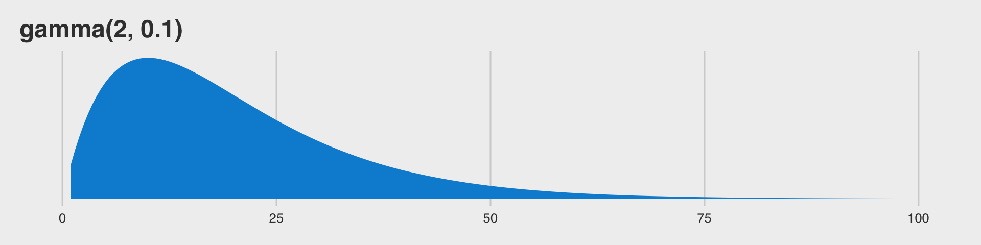
So gamma(2, 0.1) should gently push the \(\nu\) posterior toward low values, but it’s slowly-sloping right tail will allow higher values to emerge.
Following the Stan team’s recommendation, the brms default and Baez-Ortega’s blog, here’s our robust Student’s \(t\) model for the x.noisy data.
f2 <-
  brm(data = x.noisy,
      family = student,
      bf(mvbind(x, y) ~ 1) + set_rescor(TRUE),
      prior = c(prior(gamma(2, .1), class = nu),
                prior(normal(0, 100), class = Intercept, resp = x),
                prior(normal(0, 100), class = Intercept, resp = y),
                prior(normal(0, 100), class = sigma, resp = x),
                prior(normal(0, 100), class = sigma, resp = y),
                prior(lkj(1), class = rescor)),
      iter = 2000, warmup = 500, chains = 4, cores = 4,
      seed = 210191)
print(f2)
##  Family: MV(student, student)
##   Links: mu = identity; sigma = identity; nu = identity
##          mu = identity; sigma = identity; nu = identity
## Formula: x ~ 1
##          y ~ 1
##    Data: x.noisy (Number of observations: 40)
##   Draws: 4 chains, each with iter = 2000; warmup = 500; thin = 1;
##          total post-warmup draws = 6000
##
## Population-Level Effects:
##             Estimate Est.Error l-95% CI u-95% CI Rhat Bulk_ESS Tail_ESS
## x_Intercept    -2.20      3.64    -9.61     4.68 1.00     2586     2921
## y_Intercept     2.13      7.23   -11.65    16.99 1.00     2704     2636
##
## Family Specific Parameters:
##         Estimate Est.Error l-95% CI u-95% CI Rhat Bulk_ESS Tail_ESS
## sigma_x    18.24      3.02    12.90    24.59 1.00     2815     3265
## sigma_y    36.34      6.01    25.90    49.35 1.00     2812     2918
## nu          2.60      0.94     1.34     4.84 1.00     3231     2359
## nu_x        1.00      0.00     1.00     1.00   NA       NA       NA
## nu_y        1.00      0.00     1.00     1.00   NA       NA       NA
##
## Residual Correlations:
##             Estimate Est.Error l-95% CI u-95% CI Rhat Bulk_ESS Tail_ESS
## rescor(x,y)    -0.93      0.03    -0.97    -0.85 1.00     3624     3511
##
## Draws were sampled using sampling(NUTS). For each parameter, Bulk_ESS
## and Tail_ESS are effective sample size measures, and Rhat is the potential
## scale reduction factor on split chains (at convergence, Rhat = 1).
Whoa, look at that correlation, rescore(x,y)! It’s right about what we’d hope for. Sure, it’s not a perfect -.95, but that’s way better than -.61.
While we’re at it, we may as well see what happens when we fit a Student’s \(t\) model when we have perfectly multivariate normal data. Here it is with the x.clean data.
f3 <-
  update(f2,
         newdata = x.clean,
         iter = 2000, warmup = 500, chains = 4, cores = 4, seed = 210191)
print(f3)
##  Family: MV(student, student)
##   Links: mu = identity; sigma = identity; nu = identity
##          mu = identity; sigma = identity; nu = identity
## Formula: x ~ 1
##          y ~ 1
##    Data: x.clean (Number of observations: 40)
##   Draws: 4 chains, each with iter = 2000; warmup = 500; thin = 1;
##          total post-warmup draws = 6000
##
## Population-Level Effects:
##             Estimate Est.Error l-95% CI u-95% CI Rhat Bulk_ESS Tail_ESS
## x_Intercept    -2.28      3.52    -9.33     4.52 1.00     2687     3065
## y_Intercept     2.58      7.01   -10.85    16.53 1.00     2664     2938
##
## Family Specific Parameters:
##         Estimate Est.Error l-95% CI u-95% CI Rhat Bulk_ESS Tail_ESS
## sigma_x    20.77      2.64    16.31    26.51 1.00     2610     2900
## sigma_y    41.33      5.28    32.38    52.63 1.00     2595     2768
## nu         22.66     13.99     5.43    57.39 1.00     3681     2568
## nu_x        1.00      0.00     1.00     1.00   NA       NA       NA
## nu_y        1.00      0.00     1.00     1.00   NA       NA       NA
##
## Residual Correlations:
##             Estimate Est.Error l-95% CI u-95% CI Rhat Bulk_ESS Tail_ESS
## rescor(x,y)    -0.96      0.02    -0.98    -0.92 1.00     3055     3315
##
## Draws were sampled using sampling(NUTS). For each parameter, Bulk_ESS
## and Tail_ESS are effective sample size measures, and Rhat is the potential
## scale reduction factor on split chains (at convergence, Rhat = 1).
So when you don’t need Student’s \(t\), it yields the right answer anyways. That’s a nice feature.
We should probably compare the posteriors of the correlations across the four models. First we’ll collect the posterior samples into a tibble.
posts <-
  tibble(model = str_c("f", 0:3)) %>%
  mutate(fit = map(model, get)) %>%
  mutate(post = map(fit, as_draws_df)) %>%
  unnest(post)

head(posts)
## # A tibble: 6 × 15
## model fit b_x_Inte…¹ b_y_I…² sigma_x sigma_y resco…³ lprior lp__ .chain
## <chr> <list> <dbl> <dbl> <dbl> <dbl> <dbl> <dbl> <dbl> <int>
## 1 f0 <brmsfit> -1.77 2.18 22.6 45.7 -0.960 -21.5 -351. 1
## 2 f0 <brmsfit> -8.00 13.3 20.7 41.7 -0.954 -21.5 -352. 1
## 3 f0 <brmsfit> -5.44 8.18 23.7 47.4 -0.967 -21.5 -352. 1
## 4 f0 <brmsfit> -3.02 5.78 21.5 42.5 -0.962 -21.5 -351. 1
## 5 f0 <brmsfit> -3.89 6.27 22.7 41.3 -0.959 -21.5 -353. 1
## 6 f0 <brmsfit> -3.64 7.21 23.7 44.8 -0.950 -21.5 -353. 1
## # … with 5 more variables: .iteration <int>, .draw <int>, nu <dbl>, nu_x <dbl>,
## # nu_y <dbl>, and abbreviated variable names ¹b_x_Intercept, ²b_y_Intercept,
## # ³rescor__x__y
With the posterior draws in hand, we just need to wrangle a bit before showing the correlation posteriors in a coefficient plot. To make things easier, we’ll do so with a couple convenience functions from the tidybayes package.
library(tidybayes)

# wrangle
posts %>%
  group_by(model) %>%
  median_qi(rescor__x__y, .width = c(.5, .95)) %>%
  mutate(key = recode(model,
                      f0 = "Gaussian likelihood with clean data",
                      f1 = "Gaussian likelihood with noisy data",
                      f2 = "Student likelihood with noisy data",
                      f3 = "Student likelihood with clean data"),
         clean = ifelse(model %in% c("f0", "f3"), "0", "1")) %>%

  # plot
  ggplot(aes(x = rescor__x__y, xmin = .lower, xmax = .upper, y = key,
             color = clean)) +
  geom_pointinterval() +
  scale_color_fivethirtyeight() +
  scale_x_continuous(breaks = -5:0 / 5, limits = -1:0, expand = expansion(mult = c(0, 0.05))) +
  labs(subtitle = expression(paste("The posterior for ", rho, " depends on the likelihood. Why not go robust and use Student's ", italic(t), "?"))) +
  theme_fivethirtyeight() +
  theme(axis.text.y = element_text(hjust = 0),
        legend.position = "none")
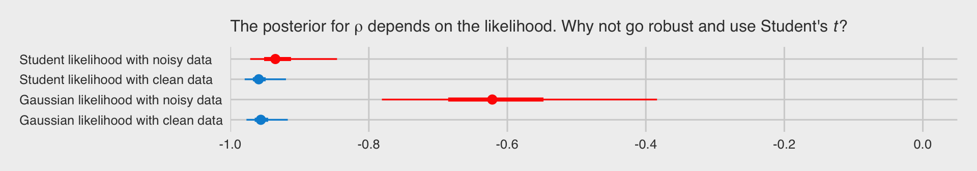
From our tidybayes::median_qi() code, the dots are the posterior medians, the thick inner lines the 50% intervals, and the thinner outer lines the 95% intervals. The posteriors for the x.noisy data are in red and those for the x.clean data are in blue. If the data are clean multivariate normal Gaussian or if they’re dirty but fit with robust Student’s \(t\), everything is pretty much alright. But whoa, if you fit a correlation with a combination of family = gaussian and noisy outlier-laden data, man that’s just a mess.
Don’t let a few overly-influential outliers make a mess of your analyses. Try the robust Student’s \(t\).
sessionInfo()
## R version 4.2.0 (2022-04-22)
## Platform: x86_64-apple-darwin17.0 (64-bit)
## Running under: macOS Big Sur/Monterey 10.16
##
## Matrix products: default
## BLAS:   /Library/Frameworks/R.framework/Versions/4.2/Resources/lib/libRblas.0.dylib
## LAPACK: /Library/Frameworks/R.framework/Versions/4.2/Resources/lib/libRlapack.dylib
##
## locale:
## [1] en_US.UTF-8/en_US.UTF-8/en_US.UTF-8/C/en_US.UTF-8/en_US.UTF-8
##
## attached base packages:
## [1] stats     graphics  grDevices utils     datasets  methods   base
##
## other attached packages:
##  [1] tidybayes_3.0.2 brms_2.18.0     Rcpp_1.0.9      ggthemes_4.2.4
##  [5] forcats_0.5.1   stringr_1.4.1   dplyr_1.0.10    purrr_0.3.4
##  [9] readr_2.1.2     tidyr_1.2.1     tibble_3.1.8    ggplot2_3.4.0
## [13] tidyverse_1.3.2 mvtnorm_1.1-3
##
## loaded via a namespace (and not attached):
##   [1] readxl_1.4.1         backports_1.4.1      Hmisc_4.7-1
##   [4] plyr_1.8.7           igraph_1.3.4         svUnit_1.0.6
##   [7] splines_4.2.0        crosstalk_1.2.0      TH.data_1.1-1
##  [10] rstantools_2.2.0     inline_0.3.19        digest_0.6.30
##  [13] htmltools_0.5.3      gdata_2.18.0.1       fansi_1.0.3
##  [16] magrittr_2.0.3       checkmate_2.1.0      cluster_2.1.3
##  [19] googlesheets4_1.0.1  tzdb_0.3.0           modelr_0.1.8
##  [22] RcppParallel_5.1.5   matrixStats_0.62.0   xts_0.12.1
##  [25] sandwich_3.0-2       prettyunits_1.1.1    jpeg_0.1-9
##  [28] colorspace_2.0-3     rvest_1.0.2          ggdist_3.2.0
##  [31] haven_2.5.1          xfun_0.35            callr_3.7.3
##  [34] crayon_1.5.2         jsonlite_1.8.3       lme4_1.1-31
##  [37] survival_3.4-0       zoo_1.8-10           glue_1.6.2
##  [40] gtable_0.3.1         gargle_1.2.0         emmeans_1.8.0
##  [43] distributional_0.3.1 weights_1.0.4        pkgbuild_1.3.1
##  [46] rstan_2.21.7         abind_1.4-5          scales_1.2.1
##  [49] DBI_1.1.3            miniUI_0.1.1.1       htmlTable_2.4.1
##  [52] xtable_1.8-4         foreign_0.8-82       Formula_1.2-4
##  [55] stats4_4.2.0         StanHeaders_2.21.0-7 DT_0.24
##  [58] htmlwidgets_1.5.4    httr_1.4.4           threejs_0.3.3
##  [61] arrayhelpers_1.1-0   RColorBrewer_1.1-3   posterior_1.3.1
##  [64] ellipsis_0.3.2       mice_3.14.0          pkgconfig_2.0.3
##  [67] loo_2.5.1            farver_2.1.1         nnet_7.3-17
##  [70] deldir_1.0-6         sass_0.4.2           dbplyr_2.2.1
##  [73] utf8_1.2.2           labeling_0.4.2       tidyselect_1.1.2
##  [76] rlang_1.0.6          reshape2_1.4.4       later_1.3.0
##  [79] munsell_0.5.0        cellranger_1.1.0     tools_4.2.0
##  [82] cachem_1.0.6         cli_3.4.1            generics_0.1.3
##  [85] broom_1.0.1          ggridges_0.5.3       evaluate_0.18
##  [88] fastmap_1.1.0        yaml_2.3.5           processx_3.8.0
##  [91] knitr_1.40           fs_1.5.2             nlme_3.1-159
##  [94] mime_0.12            projpred_2.2.1       xml2_1.3.3
##  [97] compiler_4.2.0       bayesplot_1.9.0      shinythemes_1.2.0
## [100] rstudioapi_0.13      png_0.1-7            gamm4_0.2-6
## [103] reprex_2.0.2         bslib_0.4.0          stringi_1.7.8
## [106] highr_0.9            ps_1.7.2             blogdown_1.15
## [109] Brobdingnag_1.2-8    lattice_0.20-45      Matrix_1.4-1
## [112] nloptr_2.0.3         markdown_1.1         shinyjs_2.1.0
## [115] tensorA_0.36.2       vctrs_0.5.0          pillar_1.8.1
## [118] lifecycle_1.0.3      jquerylib_0.1.4      bridgesampling_1.1-2
## [121] estimability_1.4.1   data.table_1.14.2    httpuv_1.6.5
## [124] latticeExtra_0.6-30  R6_2.5.1             bookdown_0.28
## [127] promises_1.2.0.1     gridExtra_2.3        codetools_0.2-18
## [130] boot_1.3-28          colourpicker_1.1.1   MASS_7.3-58.1
## [133] gtools_3.9.3         assertthat_0.2.1     withr_2.5.0
## [136] shinystan_2.6.0      multcomp_1.4-20      mgcv_1.8-40
## [139] parallel_4.2.0       hms_1.1.1            rpart_4.1.16
## [142] grid_4.2.0           coda_0.19-4          minqa_1.2.5
## [145] rmarkdown_2.16       googledrive_2.0.0    shiny_1.7.2
## [148] lubridate_1.8.0      base64enc_0.1-3      dygraphs_1.1.1.6
## [151] interp_1.1-3
- Posted on:
- February 10, 2019
- Length:
- 16 minute read, 3369 words