Would you like all your posteriors in one plot?
By A. Solomon Kurz
July 13, 2019
[edited on Dec 11, 2022]
A colleague reached out to me earlier this week with a plotting question. They had fit a series of Bayesian models, all containing a common parameter of interest. They knew how to plot their focal parameter one model at a time, but were stumped on how to combine the plots across models into a seamless whole. It reminded me a bit of this gif

which I originally got from Jenny Bryan’s great talk, Behind every great plot there’s a great deal of wrangling.
The goal of this post is to provide solutions. We’ll practice a few different ways you can combine the posterior samples from your Bayesian models into a single plot. As usual, we’ll be fitting our models with brms, wrangling with packages from the tidyverse, and getting a little help from the tidybayes package.
I make assumptions.
For this post, I’m presuming you are familiar Bayesian regression using brms. I’m also assuming you’ve coded using some of the foundational functions from the tidyverse. If you’d like to firm up your foundations a bit, check out these resources.
- To learn about Bayesian regression, I recommend the introductory text books by either McElreath ( here) or Kruschke ( here). Both authors host blogs ( here and here, respectively). If you go with McElreath, do check out his online lectures and my ebooks where I translated his text to brms and tidyverse code ( here and here). I have a similar ebook translation for Kruschke’s text ( here).
- For even more brms-related resources, you can find vignettes and documentation here.
- For tidyverse introductions, your best bets are R4DS and The tidyverse style guide.
Same parameter, different models
Let’s load our primary statistical packages.
library(tidyverse)
library(brms)
library(tidybayes)
Simulate \(n = 150\) draws from the standard normal distribution.
n <- 150

set.seed(1)
d <- tibble(y = rnorm(n, mean = 0, sd = 1))

head(d)
## # A tibble: 6 × 1
##        y
##    <dbl>
## 1 -0.626
## 2  0.184
## 3 -0.836
## 4  1.60
## 5  0.330
## 6 -0.820
Here we’ll fit three intercept-only models for y. Each will follow the form
$$
\begin{align*} y_i & \sim \text{Normal} (\mu, \sigma) \\ \mu & = \beta_0 \\ \beta_0 & \sim \text{Normal} (0, x) \\ \sigma & \sim \text{Student-t}(3, 0, 10) \end{align*}
$$
where \(\beta_0\) is the unconditional intercept (i.e., an intercept not conditioned on any predictors). We will be fitting three alternative models. All will have the same prior for \(\sigma\), \(\text{Student-t}(3, 0, 10)\), which is the brms default in this case. [If you’d like to check, use the get_prior() function.] The only way the models will differ is by their prior on the intercept \(\beta_0\). By model, those priors will be
fit1:\(\beta_0 \sim \text{Normal} (0, 10)\),fit2:\(\beta_0 \sim \text{Normal} (0, 1)\), andfit3:\(\beta_0 \sim \text{Normal} (0, 0.1)\).
So if you were wondering, the \(x\) in the \(\beta_0 \sim \text{Normal} (0, x)\) line, above, was a stand-in for the varying
hyperparameter.
Here we fit the models in bulk.
fit1 <-
  brm(data = d,
      family = gaussian,
      y ~ 1,
      prior(normal(0, 10), class = Intercept),
      seed = 1)

fit2 <-
  update(fit1,
         prior = prior(normal(0, 1), class = Intercept),
         seed = 1)

fit3 <-
  update(fit1,
         prior = prior(normal(0, 0.1), class = Intercept),
         seed = 1)
Normally we’d use plot() to make sure the chains look good and then use something like print() or posterior_summary() to summarize the models’ results. I’ve checked and they’re all fine. For the sake of space, let’s press forward.
If you were going to plot the results of an individual fit using something like the tidybayes::stat_halfeye() function, the next step would be extracting the posterior draws. Here we’ll do so with the brms::as_draws_df() function.
draws1 <- as_draws_df(fit1)
draws2 <- as_draws_df(fit2)
draws3 <- as_draws_df(fit3)
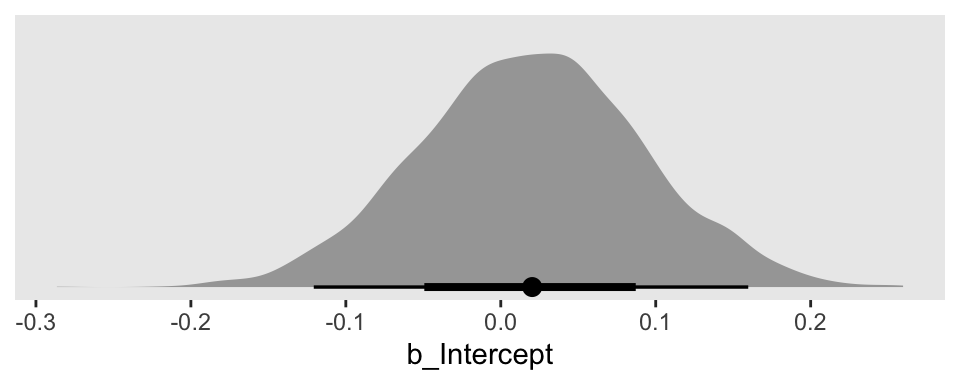
Focusing on fit1, here’s how we’d plot the results for the intercept \(\beta_0\).
# this part is unnecessary; it just adjusts some theme defaults to my liking
theme_set(theme_gray() +
            theme(axis.text.y  = element_text(hjust = 0),
                  axis.ticks.y = element_blank(),
                  panel.grid   = element_blank()))

# plot!
draws1 %>%
  ggplot(aes(x = b_Intercept, y = 0)) +
  stat_halfeye() +
  scale_y_continuous(NULL, breaks = NULL)
But how might we get the posterior draws from all three fits into one plot? The answer is by somehow combining the posterior draws from each into one data frame. There are many ways to do this. Perhaps the simplest is with the bind_rows() function.
draws <-
  bind_rows(
    draws1,
    draws2,
    draws3
  ) %>%
  mutate(prior = str_c("normal(0, ", c(10, 1, 0.1), ")") %>% rep(., each = 4000))

glimpse(draws)
## Rows: 12,000
## Columns: 8
## $ b_Intercept <dbl> 0.109776777, 0.071063836, 0.071063836, -0.018918739, -0.107746369, 0.043480309…
## $ sigma       <dbl> 0.9443561, 0.7580639, 0.7580639, 0.9125649, 0.9658271, 0.8645181, 0.8630736, 0…
## $ lprior      <dbl> -4.538550, -4.505958, -4.505958, -4.532471, -4.542719, -4.523739, -4.523486, -…
## $ lp__        <dbl> -202.7961, -207.3802, -207.3802, -202.0266, -203.8443, -202.2125, -202.2615, -…
## $ .chain      <int> 1, 1, 1, 1, 1, 1, 1, 1, 1, 1, 1, 1, 1, 1, 1, 1, 1, 1, 1, 1, 1, 1, 1, 1, 1, 1, …
## $ .iteration  <int> 1, 2, 3, 4, 5, 6, 7, 8, 9, 10, 11, 12, 13, 14, 15, 16, 17, 18, 19, 20, 21, 22,…
## $ .draw       <int> 1, 2, 3, 4, 5, 6, 7, 8, 9, 10, 11, 12, 13, 14, 15, 16, 17, 18, 19, 20, 21, 22,…
## $ prior       <chr> "normal(0, 10)", "normal(0, 10)", "normal(0, 10)", "normal(0, 10)", "normal(0,…
The bind_rows() function worked well, here, because all three post objects had the same number of columns of the same names. So we just stacked them three high. That is, we went from three data objects of 4,000 rows and 3 columns to one data object with 12,000 rows and 3 columns. But with the mutate() function we did add a fourth column, prior, that indexed which model each row came from. Now our data are ready, we can plot.
draws %>%
  ggplot(aes(x = b_Intercept, y = prior)) +
  stat_halfeye()
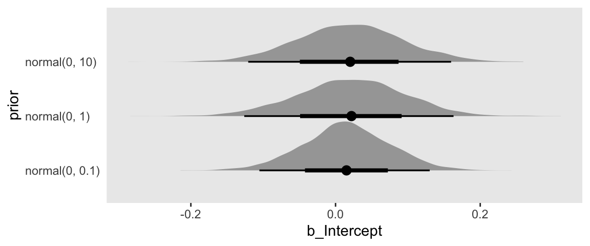
Our plot arrangement made it easy to compare the results of tightening the prior on \(\beta_0\); the narrower the prior, the narrower the posterior.
What if my as_draws_df()’s aren’t of the same dimensions across models?
For the next examples, we need new data. Here we’ll simulate three predictors–x1, x2, and x3. We then simulate our criterion y as a linear additive function of those predictors.
set.seed(1)
d <-
  tibble(x1 = rnorm(n, mean = 0, sd = 1),
         x2 = rnorm(n, mean = 0, sd = 1),
         x3 = rnorm(n, mean = 0, sd = 1)) %>%
  mutate(y  = rnorm(n, mean = 0 + x1 * 0 + x2 * 0.2 + x3 * -0.4))

head(d)
## # A tibble: 6 × 4
##       x1      x2     x3      y
##    <dbl>   <dbl>  <dbl>  <dbl>
## 1 -0.626  0.450   0.894  0.694
## 2  0.184 -0.0186 -1.05  -0.189
## 3 -0.836 -0.318   1.97  -1.61
## 4  1.60  -0.929  -0.384 -1.59
## 5  0.330 -1.49    1.65  -2.41
## 6 -0.820 -1.08    1.51  -0.764
We are going to work with these data in two ways. For the first example, we’ll fit a series of univariable models following the same basic form, but each with a different predictor. For the second example, we’ll fit a series of multivariable models with various combinations of the predictors. Each requires its own approach.
Same form, different predictors.
This time we’re just using the brms default priors. As such, the models all follow the form
$$
\begin{align*} y_i & \sim \text{Normal} (\mu_i, \sigma) \\ \mu_i & = \beta_0 + \beta_n x_n\\ \beta_0 & \sim \text{Student-t}(3, 0, 10) \\ \sigma & \sim \text{Student-t}(3, 0, 10) \end{align*}
$$
You may be wondering What about the prior for \(\beta_n\)? The brms defaults for those are improper flat priors. We define \(\beta_n x_n\) for the next three models as
fit4:\(\beta_1 x_1\),fit5:\(\beta_2 x_2\), andfit5:\(\beta_3 x_3\).
Let’s fit the models.
fit4 <-
  brm(data = d,
      family = gaussian,
      y ~ 1 + x1,
      seed = 1)

fit5 <-
  update(fit4,
         newdata = d,
         y ~ 1 + x2,
         seed = 1)

fit6 <-
  update(fit4,
         newdata = d,
         y ~ 1 + x3,
         seed = 1)
Like before, save the posterior draws for each as separate data frames.
draws4 <- as_draws_df(fit4)
draws5 <- as_draws_df(fit5)
draws6 <- as_draws_df(fit6)
This time, our simple bind_rows() trick won’t work well.
bind_rows(
  draws4,
  draws5,
  draws6
) %>%
  head()
## # A draws_df: 6 iterations, 1 chains, and 7 variables
##   b_Intercept   b_x1 sigma lprior lp__ b_x2 b_x3
## 1       0.091 -0.093   1.2   -3.3 -240   NA   NA
## 2       0.081 -0.083   1.2   -3.3 -239   NA   NA
## 3       0.031 -0.255   1.3   -3.3 -241   NA   NA
## 4       0.084  0.059   1.2   -3.3 -241   NA   NA
## 5      -0.076 -0.203   1.2   -3.3 -240   NA   NA
## 6      -0.057 -0.098   1.1   -3.3 -240   NA   NA
## # ... hidden reserved variables {'.chain', '.iteration', '.draw'}
We don’t want separate columns for b_x1, b_x2, and b_x3. We want them all stacked atop one another. One simple solution is a two-step wherein we (1) select the relevant columns from each and bind them together with bind_cols() and then (2) stack them atop one another with the gather() function.
draws <-
  bind_cols(
    draws4 %>% select(b_x1),
    draws5 %>% select(b_x2),
    draws6 %>% select(b_x3)
  ) %>%
  gather() %>%
  mutate(predictor = str_remove(key, "b_"))

head(draws)
## # A tibble: 6 × 3
##   key     value predictor
##   <chr>   <dbl> <chr>
## 1 b_x1  -0.0933 x1
## 2 b_x1  -0.0826 x1
## 3 b_x1  -0.255  x1
## 4 b_x1   0.0591 x1
## 5 b_x1  -0.203  x1
## 6 b_x1  -0.0977 x1
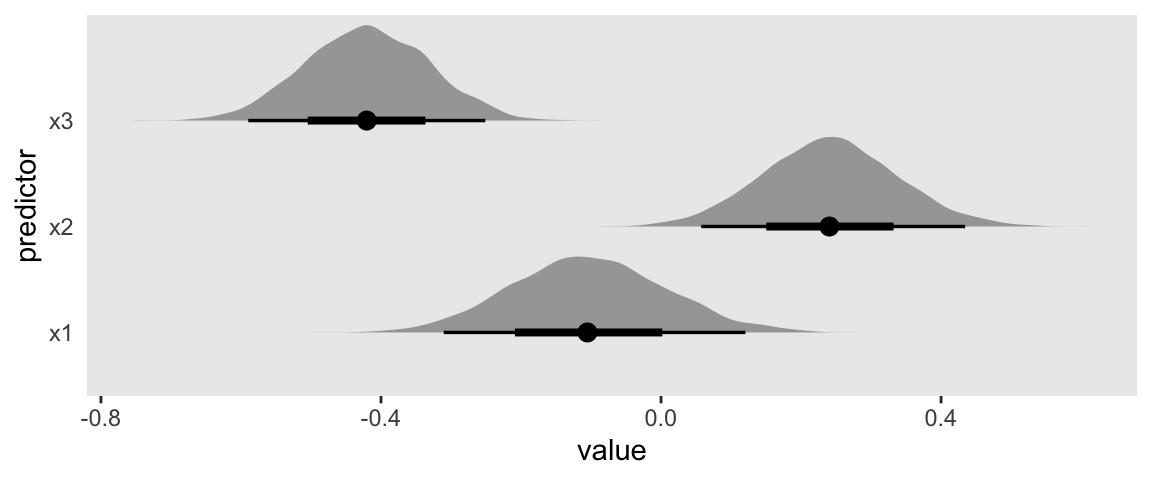
That mutate() line at the end wasn’t necessary, but it will make the plot more attractive.
draws %>%
  ggplot(aes(x = value, y = predictor)) +
  stat_halfeye()
Different combinations of predictors in different forms.
Now we fit a series of multivariable models. The first three will have combinations of two of the predictors. The final model will have all three. For simplicity, we continue to use the brms default priors.
fit7 <-
  brm(data = d,
      family = gaussian,
      y ~ 1 + x1 + x2,
      seed = 1)

fit8 <-
  update(fit7,
         newdata = d,
         y ~ 1 + x1 + x3,
         seed = 1)

fit9 <-
  update(fit7,
         newdata = d,
         y ~ 1 + x2 + x3,
         seed = 1)

fit10 <-
  update(fit7,
         newdata = d,
         y ~ 1 + x1 + x2 + x3,
         seed = 1)
Individually extract the posterior draws.
draws7  <- as_draws_df(fit7)
draws8  <- as_draws_df(fit8)
draws9  <- as_draws_df(fit9)
draws10 <- as_draws_df(fit10)
Take a look at what happens this time when we use the bind_rows() approach.
draws <-
  bind_rows(
    draws7,
    draws8,
    draws9,
    draws10
  )

glimpse(draws)
## Rows: 16,000
## Columns: 10
## $ b_Intercept <dbl> 0.121129174, 0.012766747, 0.082335019, -0.166668199, 0.041276697, 0.036409424,…
## $ b_x1        <dbl> -0.111236289, -0.087489940, -0.257404363, -0.199365456, -0.043018776, -0.06762…
## $ b_x2        <dbl> 0.29084052, 0.14044206, 0.21107496, 0.24211793, 0.20718236, 0.15167782, 0.3214…
## $ sigma       <dbl> 1.109546, 1.121134, 1.108340, 1.117748, 1.084008, 1.135944, 1.189880, 1.114291…
## $ lprior      <dbl> -3.274126, -3.272449, -3.271829, -3.270609, -3.265173, -3.276466, -3.289609, -…
## $ lp__        <dbl> -237.0847, -236.3169, -237.6600, -237.7328, -236.4454, -236.2540, -237.6852, -…
## $ .chain      <int> 1, 1, 1, 1, 1, 1, 1, 1, 1, 1, 1, 1, 1, 1, 1, 1, 1, 1, 1, 1, 1, 1, 1, 1, 1, 1, …
## $ .iteration  <int> 1, 2, 3, 4, 5, 6, 7, 8, 9, 10, 11, 12, 13, 14, 15, 16, 17, 18, 19, 20, 21, 22,…
## $ .draw       <int> 1, 2, 3, 4, 5, 6, 7, 8, 9, 10, 11, 12, 13, 14, 15, 16, 17, 18, 19, 20, 21, 22,…
## $ b_x3        <dbl> NA, NA, NA, NA, NA, NA, NA, NA, NA, NA, NA, NA, NA, NA, NA, NA, NA, NA, NA, NA…
We still have the various data frames stacked atop another, with the data from draws7 in the first 4,000 rows. See how the values in the b_x3 column are all missing (i.e., filled with NA values)? That’s because fit7 didn’t contain x3 as a predictor. Similarly, if we were to look at rows 4,001 through 8,000, we’d see column b_x2 would be the one filled with NAs. This behavior is a good thing, here. After a little more wrangling, we’ll plot and it should be become clear why. Here’s the wrangling.
draws <-
  draws %>%
  select(starts_with("b_x")) %>%
  mutate(contains = rep(c("<1, 1, 0>", "<1, 0, 1>", "<0, 1, 1>", "<1, 1, 1>"), each = 4000)) %>%
  gather(key, value, -contains) %>%
  mutate(coefficient = str_remove(key, "b_x") %>% str_c("beta[", ., "]"))

head(draws)
## # A tibble: 6 × 4
##   contains  key     value coefficient
##   <chr>     <chr>   <dbl> <chr>
## 1 <1, 1, 0> b_x1  -0.111  beta[1]
## 2 <1, 1, 0> b_x1  -0.0875 beta[1]
## 3 <1, 1, 0> b_x1  -0.257  beta[1]
## 4 <1, 1, 0> b_x1  -0.199  beta[1]
## 5 <1, 1, 0> b_x1  -0.0430 beta[1]
## 6 <1, 1, 0> b_x1  -0.0676 beta[1]
With the contains variable, we indexed which fit the draws came from. The 1’s and 0’s within the angle brackets indicate which of the three predictors were present within the model with the 1’s indicating they were and the 0’s indicating they were not. For example, <1, 1, 0> in the first row indicated this was the model including x1 and x2. Importantly, we also added a coefficient index. This is just a variant of key that’ll make the strip labels in our plot more attractive. Behold:
draws %>%
  drop_na(value) %>%
  ggplot(aes(x = value, y = contains)) +
  stat_halfeye() +
  ylab(NULL) +
  facet_wrap(~coefficient, ncol = 1, labeller = label_parsed)
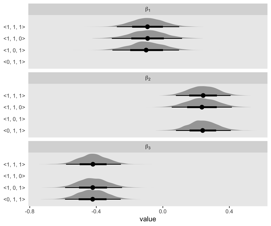
Hopefully now it’s clear why it was good to save those cells with the NAs.
Bonus: You can streamline your workflow.
The workflows above are generally fine. But they’re a little inefficient. If you’d like to reduce the amount of code you’re writing and the number of objects you have floating around in your environment, you might consider a more streamlined workflow where you work with your fit objects in bulk. Here we’ll demonstrate a nested tibble approach with the first three fits.
draws <-
  tibble(name  = str_c("fit", 1:3),
         prior = str_c("normal(0, ", c(10, 1, 0.1), ")")) %>%
  mutate(fit = map(name, get)) %>%
  mutate(draws = map(fit, as_draws_df))

head(draws)
## # A tibble: 3 × 4
##   name  prior          fit       draws
##   <chr> <chr>          <list>    <list>
## 1 fit1  normal(0, 10)  <brmsfit> <draws_df [4,000 × 7]>
## 2 fit2  normal(0, 1)   <brmsfit> <draws_df [4,000 × 7]>
## 3 fit3  normal(0, 0.1) <brmsfit> <draws_df [4,000 × 7]>
We have a 3-row nested tibble. The first column, name is just a character vector with the names of the fits. The next column isn’t necessary, but it nicely explicates the main difference in the models: the prior we used on the intercept. It’s in the map() functions within the two mutate()lines where all the magic happens. With the first, we used the get() function to snatch up the brms fit objects matching the names in the name column. In the second, we used the as_draws_df() function to extract the posterior draws from each of the fits saved in fit. Do you see how each for in the draws column contains an entire \(4,000 \times 3\) data frame? That’s why we refer to this as a nested tibble. We have data frames compressed within data frames. If you’d like to access the data within the draws column, just unnest().
draws %>%
  select(-fit) %>%
  unnest(draws)
## # A tibble: 12,000 × 9
##    name  prior         b_Intercept sigma lprior  lp__ .chain .iteration .draw
##    <chr> <chr>               <dbl> <dbl>  <dbl> <dbl>  <int>      <int> <int>
##  1 fit1  normal(0, 10)      0.110  0.944  -4.54 -203.      1          1     1
##  2 fit1  normal(0, 10)      0.0711 0.758  -4.51 -207.      1          2     2
##  3 fit1  normal(0, 10)      0.0711 0.758  -4.51 -207.      1          3     3
##  4 fit1  normal(0, 10)     -0.0189 0.913  -4.53 -202.      1          4     4
##  5 fit1  normal(0, 10)     -0.108  0.966  -4.54 -204.      1          5     5
##  6 fit1  normal(0, 10)      0.0435 0.865  -4.52 -202.      1          6     6
##  7 fit1  normal(0, 10)      0.0486 0.863  -4.52 -202.      1          7     7
##  8 fit1  normal(0, 10)      0.0217 0.911  -4.53 -202.      1          8     8
##  9 fit1  normal(0, 10)      0.0244 0.880  -4.53 -202.      1          9     9
## 10 fit1  normal(0, 10)     -0.0497 0.860  -4.52 -203.      1         10    10
## # … with 11,990 more rows
After un-nesting, we can remake the plot from above.
draws %>%
  select(-fit) %>%
  unnest(draws) %>%

  ggplot(aes(x = b_Intercept, y = prior)) +
  stat_halfeye()

To learn more about using the tidyverse for iterating and saving the results in nested tibbles, check out Hadley Wickham’s great talk, Managing many models.
Session information
sessionInfo()
## R version 4.2.0 (2022-04-22)
## Platform: x86_64-apple-darwin17.0 (64-bit)
## Running under: macOS Big Sur/Monterey 10.16
##
## Matrix products: default
## BLAS:   /Library/Frameworks/R.framework/Versions/4.2/Resources/lib/libRblas.0.dylib
## LAPACK: /Library/Frameworks/R.framework/Versions/4.2/Resources/lib/libRlapack.dylib
##
## locale:
## [1] en_US.UTF-8/en_US.UTF-8/en_US.UTF-8/C/en_US.UTF-8/en_US.UTF-8
##
## attached base packages:
## [1] stats     graphics  grDevices utils     datasets  methods   base
##
## other attached packages:
##  [1] tidybayes_3.0.2 brms_2.18.0     Rcpp_1.0.9      forcats_0.5.1   stringr_1.4.1   dplyr_1.0.10
##  [7] purrr_0.3.4     readr_2.1.2     tidyr_1.2.1     tibble_3.1.8    ggplot2_3.4.0   tidyverse_1.3.2
##
## loaded via a namespace (and not attached):
##   [1] readxl_1.4.1         backports_1.4.1      plyr_1.8.7           igraph_1.3.4
##   [5] svUnit_1.0.6         splines_4.2.0        crosstalk_1.2.0      TH.data_1.1-1
##   [9] rstantools_2.2.0     inline_0.3.19        digest_0.6.30        htmltools_0.5.3
##  [13] fansi_1.0.3          magrittr_2.0.3       checkmate_2.1.0      googlesheets4_1.0.1
##  [17] tzdb_0.3.0           modelr_0.1.8         RcppParallel_5.1.5   matrixStats_0.62.0
##  [21] xts_0.12.1           sandwich_3.0-2       prettyunits_1.1.1    colorspace_2.0-3
##  [25] rvest_1.0.2          ggdist_3.2.0         haven_2.5.1          xfun_0.35
##  [29] callr_3.7.3          crayon_1.5.2         jsonlite_1.8.3       lme4_1.1-31
##  [33] survival_3.4-0       zoo_1.8-10           glue_1.6.2           gtable_0.3.1
##  [37] gargle_1.2.0         emmeans_1.8.0        distributional_0.3.1 pkgbuild_1.3.1
##  [41] rstan_2.21.7         abind_1.4-5          scales_1.2.1         mvtnorm_1.1-3
##  [45] DBI_1.1.3            miniUI_0.1.1.1       xtable_1.8-4         stats4_4.2.0
##  [49] StanHeaders_2.21.0-7 DT_0.24              htmlwidgets_1.5.4    httr_1.4.4
##  [53] threejs_0.3.3        arrayhelpers_1.1-0   posterior_1.3.1      ellipsis_0.3.2
##  [57] pkgconfig_2.0.3      loo_2.5.1            farver_2.1.1         sass_0.4.2
##  [61] dbplyr_2.2.1         utf8_1.2.2           labeling_0.4.2       tidyselect_1.1.2
##  [65] rlang_1.0.6          reshape2_1.4.4       later_1.3.0          munsell_0.5.0
##  [69] cellranger_1.1.0     tools_4.2.0          cachem_1.0.6         cli_3.4.1
##  [73] generics_0.1.3       broom_1.0.1          ggridges_0.5.3       evaluate_0.18
##  [77] fastmap_1.1.0        yaml_2.3.5           processx_3.8.0       knitr_1.40
##  [81] fs_1.5.2             nlme_3.1-159         mime_0.12            projpred_2.2.1
##  [85] xml2_1.3.3           compiler_4.2.0       bayesplot_1.9.0      shinythemes_1.2.0
##  [89] rstudioapi_0.13      gamm4_0.2-6          reprex_2.0.2         bslib_0.4.0
##  [93] stringi_1.7.8        highr_0.9            ps_1.7.2             blogdown_1.15
##  [97] Brobdingnag_1.2-8    lattice_0.20-45      Matrix_1.4-1         nloptr_2.0.3
## [101] markdown_1.1         shinyjs_2.1.0        tensorA_0.36.2       vctrs_0.5.0
## [105] pillar_1.8.1         lifecycle_1.0.3      jquerylib_0.1.4      bridgesampling_1.1-2
## [109] estimability_1.4.1   httpuv_1.6.5         R6_2.5.1             bookdown_0.28
## [113] promises_1.2.0.1     gridExtra_2.3        codetools_0.2-18     boot_1.3-28
## [117] colourpicker_1.1.1   MASS_7.3-58.1        gtools_3.9.3         assertthat_0.2.1
## [121] withr_2.5.0          shinystan_2.6.0      multcomp_1.4-20      mgcv_1.8-40
## [125] parallel_4.2.0       hms_1.1.1            grid_4.2.0           coda_0.19-4
## [129] minqa_1.2.5          rmarkdown_2.16       googledrive_2.0.0    shiny_1.7.2
## [133] lubridate_1.8.0      base64enc_0.1-3      dygraphs_1.1.1.6
- Posted on:
- July 13, 2019
- Length:
- 15 minute read, 3046 words