Bayesian power analysis: Part I. Prepare to reject `\(H_0\)` with simulation.
By A. Solomon Kurz
July 18, 2019
Version 1.1.0
Edited on April 21, 2021, to remove the broom::tidy() portion of the workflow.
tl;dr
If you’d like to learn how to do Bayesian power calculations using brms, stick around for this multi-part blog series. Here with part I, we’ll set the foundation.
Power is hard, especially for Bayesians.
Many journals, funding agencies, and dissertation committees require power calculations for your primary analyses. Frequentists have a variety of tools available to perform these calculations (e.g.,
here). Bayesians, however, have a more difficult time of it. Most of our research questions and data issues are sufficiently complicated that we cannot solve the problems by hand. We need Markov chain Monte Carlo methods to iteratively sample from the posterior to summarize the parameters from our models. Same deal for power. If you’d like to compute the power for a given combination of \(N\), likelihood \(p(\text{data} | \theta)\), and set of priors \(p (\theta)\), you’ll need to simulate.
It’s been one of my recent career goals to learn how to do this. You know how they say: The best way to learn is to teach. This series of blog posts is the evidence of me learning by teaching. It will be an exploration of what a Bayesian power simulation workflow might look like. The overall statistical framework will be within R ( R Core Team, 2022), with an emphasis on code style based on the tidyverse ( Wickham et al., 2019; Wickham, 2022). We’ll be fitting our Bayesian models with Bürkner’s brms package ( Bürkner, 2017, 2018, 2022).
What this series is not, however, is an introduction to statistical power itself. Keep reading if you’re ready to roll up your sleeves, put on your applied hat, and learn how to get things done. If you’re more interested in introductions to power, see the references in the next section.
I make assumptions.
For this series, I’m presuming you are familiar with linear regression, familiar with the basic differences between frequentist and Bayesian approaches to statistics, and have a basic sense of what we mean by statistical power. Here are some resources if you’d like to shore up.
- If you’re unfamiliar with statistical power, Kruschke covered it in chapter 13 of his ( 2015) text. You might also check out the ( 2008) review paper by Maxwell, Kelley, and Rausch. There’s always, of course, the original work by Cohen (e.g., Cohen, 1988). You might also like this Khan Academy video.
- To learn about Bayesian regression, I recommend the introductory text books by either McElreath ( 2020, 2015) or Kruschke ( 2015). Both authors host blogs ( here and here, respectively). If you go with McElreath, do check out his online lectures and my ( 2020, 2020) ebooks translating his text to brms and tidyverse code. I have an ebook for Kruschke’s text ( Kurz, 2020), too.
- For even more brms-related resources, you can find vignettes and documentation at https://cran.r-project.org/package=brms/index.html.
- For tidyverse introductions, your best bets are Grolemund and Wickham’s ( 2017) R for data science and Wickham’s ( 2020) The tidyverse style guide.
- We’ll be simulating data. If that’s new to you, both Kruschke and McElreath cover that a little in their texts. You can find nice online tutorials here and here, too.
- We’ll also be making a couple custom functions. If that’s new, you might check out R4DS, chapter 19 or chapter 14 of Roger Peng’s ( 2019) R Programming for Data Science.
We need to warm up before jumping into power.
Let’s load our primary packages. The tidyverse helps organize data and we model with brms.
library(tidyverse)
library(brms)
Consider a case where you have some dependent variable \(Y\) that you’d like to compare between two groups, which we’ll call treatment and control. Here we presume \(Y\) is continuous and, for the sake of simplicity, is in a standardized metric for the control condition. Letting \(c\) stand for control and \(i\) index the data row for a given case, we might write that as \(y_{i, c} \sim \operatorname{Normal} (0, 1)\). The mean for our treatment condition is 0.5, with the standard deviation still in the standardized metric. In the social sciences a standardized mean difference of 0.5 would typically be considered a medium effect size. Here’s what that’d look like.
# set our theme because, though I love the default ggplot theme, I hate gridlines
theme_set(theme_grey() +
            theme(panel.grid = element_blank()))

# define the means
mu_c <- 0
mu_t <- 0.5

# set up the data
tibble(x = seq(from = -4, to = 5, by = .01)) %>%
  mutate(c = dnorm(x, mean = mu_c, sd = 1),
         t = dnorm(x, mean = mu_t, sd = 1)) %>%

  # plot
  ggplot(aes(x = x)) +
  geom_area(aes(y = c),
            size = 0, alpha = 1/3, fill = "grey25") +
  geom_area(aes(y = t),
            size = 0, alpha = 1/3, fill = "blue2") +
 annotate(geom = "text",
           x = c(-.5, 1), y = .385,
           label = c("control", "treatment"),
           hjust = 1:0,
           size = 5) +
  scale_x_continuous(NULL, breaks = -4:5) +
  scale_y_continuous(NULL, breaks = NULL) +
  scale_color_manual(values = c("grey25", "blue2"))
## Warning: Using `size` aesthetic for lines was deprecated in ggplot2 3.4.0.
## ℹ Please use `linewidth` instead.
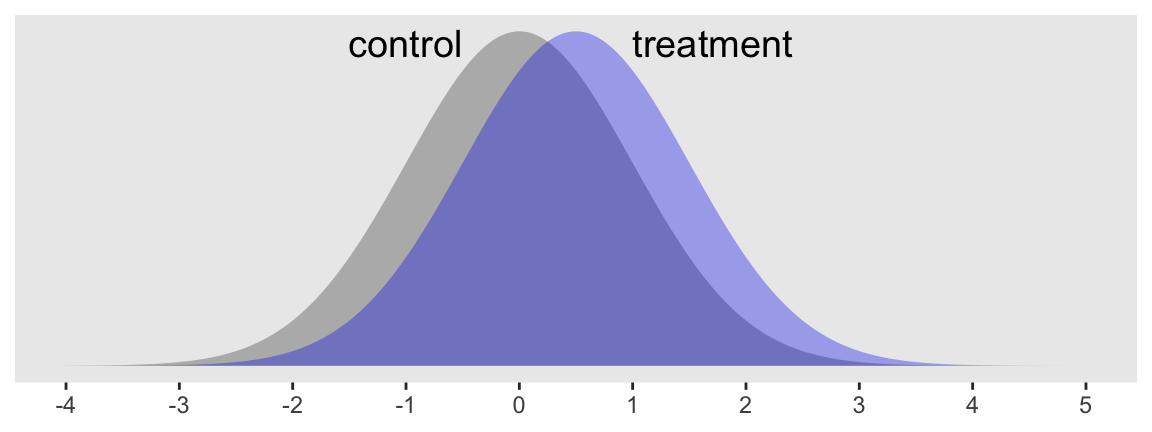
Sure, those distributions have a lot of overlap. But their means are clearly different and we’d like to make sure we plan on collecting enough data to do a good job showing that. A power analysis will help.
Within the conventional frequentist paradigm, power is the probability of rejecting the null hypothesis \(H_0\) in favor of the alternative hypothesis \(H_1\), given the alternative hypothesis is “true.” In this case, the typical null hypothesis is
$$H_0\text{: } \mu_c = \mu_t,$$
or put differently,
$$ H_0\text{: } \mu_t - \mu_c = 0. $$
And the alternative hypothesis is often just
$$H_1\text{: } \mu_c \neq \mu_t,$$
or otherwise put,
$$ H_1\text{: } \mu_t - \mu_c \neq 0. $$
Within the regression framework, we’ll be comparing \(\mu\)s using the formula
$$
\begin{align*} y_i & \sim \operatorname{Normal}(\mu_i, \sigma) \\ \mu_i & = \beta_0 + \beta_1 \text{treatment}_i, \end{align*}
$$
where \(\text{treatment}\) is a dummy variable coded 0 = control 1 = treatment and varies across cases indexed by \(i\). In this setup, \(\beta_0\) is the estimate for \(\mu_c\) and \(\beta_1\) is the estimate of the difference between condition means, \(\mu_t - \mu_c\). Thus our focal parameter, the one we care about the most in our power analysis, will be \(\beta_1\).
Within the frequentist paradigm, we typically compare these hypotheses using a \(p\)-value for \(H_0\) with the critical value, \(\alpha\), set to .05. Thus, power is the probability we’ll have \(p < .05\) when it is indeed the case that \(\mu_c \neq \mu_t\). We won’t be computing \(p\)-values in this project, but we will use 95% intervals. Recall that the result of a Bayesian analysis, the posterior distribution, is the probability of the parameters, given the data \(p (\theta | \text{data})\). With our 95% Bayesian credible intervals, we’ll be able to describe the parameter space over which our estimate of \(\mu_t - \mu_c\) is 95% probable. That is, for our power analysis, we’re interested in the probability our 95% credible intervals for \(\beta_1\) contain zero within their bounds when we know a priori \(\mu_c \neq \mu_t\).
The reason we know \(\mu_c \neq \mu_t\) is because we’ll be simulating the data that way. What our power analysis will help us determine is how many cases we’ll need to achieve a predetermined level of power. The conventional threshold is .8.
Dry run number 1.
To make this all concrete, let’s start with a simple example. We’ll simulate a single set of data, fit a Bayesian regression model, and examine the results for the critical parameter \(\beta_1\). For the sake of simplicity, let’s keep our two groups, treatment and control, the same size. We’ll start with \(n = 50\) for each.
n <- 50
We already decided above that
$$
\begin{align*} y_{i, c} & \sim \operatorname{Normal}(0, 1) \text{ and} \\ y_{i, t} & \sim \operatorname{Normal}(0.5, 1). \end{align*}
$$
Here’s how we might simulate data along those lines.
set.seed(1)

d <-
  tibble(group = rep(c("control", "treatment"), each = n)) %>%
  mutate(treatment = ifelse(group == "control", 0, 1),
         y         = ifelse(group == "control",
                            rnorm(n, mean = mu_c, sd = 1),
                            rnorm(n, mean = mu_t, sd = 1)))

glimpse(d)
## Rows: 100
## Columns: 3
## $ group     <chr> "control", "control", "control", "control", "control", "cont…
## $ treatment <dbl> 0, 0, 0, 0, 0, 0, 0, 0, 0, 0, 0, 0, 0, 0, 0, 0, 0, 0, 0, 0, …
## $ y         <dbl> -0.62645381, 0.18364332, -0.83562861, 1.59528080, 0.32950777…
In case it wasn’t clear, the two variables group and treatment are redundant. Whereas the former is composed of names, the latter is the dummy-variable equivalent (i.e., control = 0, treatment = 1). The main event was how we used the rnorm() function to simulate the normally-distributed values for y.
Before we fit our model, we need to decide on priors. To give us ideas, here are the brms defaults for our model and data.
get_prior(data = d,
          family = gaussian,
          y ~ 0 + Intercept + treatment)
##                 prior class      coef group resp dpar nlpar lb ub       source
##                (flat)     b                                            default
##                (flat)     b Intercept                             (vectorized)
##                (flat)     b treatment                             (vectorized)
##  student_t(3, 0, 2.5) sigma                                  0         default
A few things: Notice that here we’re using the 0 + Intercept syntax. This is because brms handles the priors for the default intercept under the presumption you’ve mean-centered all your predictor variables. However, since our treatment variable is a dummy, that assumption won’t fly. The 0 + Intercept allows us to treat the model intercept as just another \(\beta\) parameter, which makes no assumptions about centering. Along those lines, you’ll notice brms currently defaults to flat priors for the \(\beta\) parameters (i.e., those for which class = b). And finally, the default prior on \(\sigma\) is moderately wide student_t(3, 0, 2.5). By default, brms also sets the left bounds for \(\sigma\) parameters at zero, making that a folded-$t$ distribution. If you’re confused by these details, spend some time with the
brms reference manual (
Bürkner, 2020), particularly the brm and brmsformula sections.
In this project, we’ll be primarily using two kinds of priors: default flat priors and weakly-regularizing priors. Hopefully flat priors are self-explanatory. They let the likelihood (data) dominate the posterior and tend to produce results similar to those from frequentist estimators.
As for weakly-regularizing priors, McElreath covered them in his text. They’re mentioned a bit in the Stan team’s
Prior Choice Recommendations wiki, and you can learn even more from Gelman, Simpson, and Betancourt’s (
2017)
The prior can only be understood in the context of the likelihood. These priors aren’t strongly informative and aren’t really representative of our research hypotheses. But they’re not as absurd as flat priors, either. Rather, with just a little bit of knowledge about the data, these priors are set to keep the MCMC chains on target. Since our y variable has a mean near zero and a standard deviation near one and since our sole predictor, treatment is a dummy, setting \(\operatorname{Normal}(0, 2)\) as the prior for both \(\beta\) parameters might be a good place to start. The prior is permissive enough that it will let likelihood dominate the posterior, but it also rules out ridiculous parts of the parameter space (e.g., a standardized mean difference of 20, an intercept of -93). And since we know the data are on the unit scale, we might just center our folded-Student-$t$ prior on one and add a gentle scale setting of one.
Feel free to disagree and use your own priors. The great thing about priors is that they can be proposed, defended, criticized and improved. The point is to settle on the priors you can defend with written reasons. Select ones you’d feel comfortable defending to a skeptical reviewer.
Here’s how we might fit the model.
fit <-
  brm(data = d,
      family = gaussian,
      y ~ 0 + Intercept + treatment,
      prior = c(prior(normal(0, 2), class = b),
                prior(student_t(3, 1, 1), class = sigma)),
      seed = 1)
Before we look at the summary, we might check the chains in a trace plot. We’re looking for “stuck” chains that don’t appear to come from a normal distribution (the chains are a profile-like view rather than histogram, allowing for inspection of dependence between samples).
plot(fit)
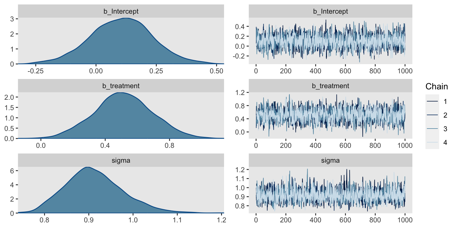
Yep, the chains all look good. Here’s the parameter summary.
print(fit)
##  Family: gaussian
##   Links: mu = identity; sigma = identity
## Formula: y ~ 0 + Intercept + treatment
##    Data: d (Number of observations: 100)
##   Draws: 4 chains, each with iter = 2000; warmup = 1000; thin = 1;
##          total post-warmup draws = 4000
##
## Population-Level Effects:
##           Estimate Est.Error l-95% CI u-95% CI Rhat Bulk_ESS Tail_ESS
## Intercept     0.11      0.13    -0.15     0.36 1.00     2159     2192
## treatment     0.51      0.18     0.15     0.87 1.00     2230     2445
##
## Family Specific Parameters:
##       Estimate Est.Error l-95% CI u-95% CI Rhat Bulk_ESS Tail_ESS
## sigma     0.91      0.07     0.80     1.06 1.00     2371     2397
##
## Draws were sampled using sampling(NUTS). For each parameter, Bulk_ESS
## and Tail_ESS are effective sample size measures, and Rhat is the potential
## scale reduction factor on split chains (at convergence, Rhat = 1).
The 95% credible intervals for our \(\beta_1\) parameter, termed treatment in the output, are well above zero.
Another way to look at the parameter summary is with the brms::fixef() function.
fixef(fit)
##            Estimate Est.Error       Q2.5     Q97.5
## Intercept 0.1052398 0.1285999 -0.1523971 0.3574843
## treatment 0.5129811 0.1827412  0.1533267 0.8742095
You can reuse a fit.
Especially with simple models like this, a lot of the time we spend waiting for brms::brm() to return the model is wrapped up in compilation. This is because brms is a collection of user-friendly functions designed to fit models with
Stan (
Stan Development Team, 2020,
2021a,
2021b). With each new model, brm() translates your model into Stan code, which then gets translated to C++ and is compiled afterwards (see
here or
here). However, we can use the update() function to update a previously-compiled fit object with new data. This cuts out the compilation time and allows us to get directly to sampling. Here’s how to do it.
# set a new seed
set.seed(2)

# simulate new data based on that new seed
d <-
  tibble(group = rep(c("control", "treatment"), each = n)) %>%
  mutate(treatment = ifelse(group == "control", 0, 1),
         y         = ifelse(group == "control",
                            rnorm(n, mean = mu_c, sd = 1),
                            rnorm(n, mean = mu_t, sd = 1)))

updated_fit <-
  update(fit,
         newdata = d,
         seed = 2)
Behold the fixef() parameter summary for our updated model.
fixef(updated_fit)
##             Estimate Est.Error       Q2.5     Q97.5
## Intercept 0.06781182 0.1702447 -0.2730871 0.3946365
## treatment 0.29955816 0.2406686 -0.1696387 0.7755439
Well how about that? In this case, our 95% credible intervals for the \(\beta_1\) treatment coefficient did include zero within their bounds. Though the posterior mean, 0.30, is still well away from zero, here we’d fail to reject \(H_0\) at the conventional level. This is why we simulate.
To recap, we’ve
- determined our primary data type,
- cast our research question in terms of a regression model,
- identified the parameter of interest,
- settled on defensible priors,
- picked an initial sample size,
- fit an initial model with a single simulated data set, and
- practiced reusing that fit with
update().
We’re more than half way there! It’s time to do our first power simulation.
Simulate to determine power.
In this post, we’ll play with three ways to do a Bayesian power simulation. They’ll all be similar, but hopefully you’ll learn a bit as we transition from one to the next. Though if you’re impatient and all this seems remedial, you could probably just skip down to the final example, Version 3.
Version 1: Let’s introduce making a custom model-fitting function.
For our power analysis, we’ll need to simulate a large number of data sets, each of which we’ll fit a model to. Here we’ll make a custom function, sim_d(), that will simulate new data sets just like before. Our function will have two parameters: we’ll set our seeds with seed and determine how many cases we’d like per group with n.
sim_d <- function(seed, n) {

  mu_t <- .5
  mu_c <- 0

  set.seed(seed)

  tibble(group = rep(c("control", "treatment"), each = n)) %>%
  mutate(treatment = ifelse(group == "control", 0, 1),
         y         = ifelse(group == "control",
                            rnorm(n, mean = mu_c, sd = 1),
                            rnorm(n, mean = mu_t, sd = 1)))
}
Here’s a quick example of how our function works.
sim_d(seed = 123, n = 2)
## # A tibble: 4 × 3
##   group     treatment      y
##   <chr>         <dbl>  <dbl>
## 1 control           0 -0.560
## 2 control           0 -0.230
## 3 treatment         1  2.06
## 4 treatment         1  0.571
Now we’re ready to get down to business. We’re going to be saving our simulation results in a nested data frame, s. Initially, s will have one column of seed values. These will serve a dual function. First, they are the values we’ll be feeding into the seed argument of our custom data-generating function, sim_d(). Second, since the seed values serially increase, they also stand in as iteration indexes.
For our second step, we add the data simulations and save them in a nested column, d. In the first argument of the purrr::map() function, we indicate we want to iterate over the values in seed. In the second argument, we indicate we want to serially plug those seed values into the first argument within the sim_d() function. That argument, recall, is the well-named seed argument. With the final argument in map(), n = 50, we hard code 50 into the n argument of sim_d().
For the third step, we expand our purrr::map() skills from above to purrr::map2(), which allows us to iteratively insert two arguments into a function. Within this paradigm, the two arguments are generically termed .x and .y. Thus our approach will be .x = d, .y = seed. For our function, we specify ~update(fit, newdata = .x, seed = .y). Thus we’ll be iteratively inserting our simulated d data into the newdata argument and will be simultaneously inserting our seed values into the seed argument.
Also notice that the number of iterations we’ll be working with is determined by the number of rows in the seed column. We are defining that number as n_sim. Since this is just a blog post, I’m going to take it easy and use 100. But if this was a real power analysis for one of your projects, something like 1,000 would be better.
Finally, you don’t have to do this, but I’m timing my simulation by saving Sys.time() values at the beginning and end of the simulation.
# how many simulations would you like?
n_sim <- 100

# this will help us track time
t1 <- Sys.time()

# here's the main event!
s <-
  tibble(seed = 1:n_sim) %>%
  mutate(d = map(seed, sim_d, n = 50)) %>%
  mutate(fit = map2(d, seed, ~update(fit, newdata = .x, seed = .y)))

t2 <- Sys.time()
The entire simulation took just about a minute on my new laptop.
t2 - t1
## Time difference of 1.383244 mins
Your mileage may vary.
Let’s take a look at what we’ve done.
head(s)
## # A tibble: 6 × 3
##    seed d                  fit
##   <int> <list>             <list>
## 1     1 <tibble [100 × 3]> <brmsfit>
## 2     2 <tibble [100 × 3]> <brmsfit>
## 3     3 <tibble [100 × 3]> <brmsfit>
## 4     4 <tibble [100 × 3]> <brmsfit>
## 5     5 <tibble [100 × 3]> <brmsfit>
## 6     6 <tibble [100 × 3]> <brmsfit>
In our 100-row nested tibble, we have all our simulated data sets in the d column and all of our brms fit objects nested in the fit column. Next we’ll use fixef() and a little wrangling to extract the parameter of interest, treatment (i.e., \(\beta_1\)), from each simulation. We’ll save the results as parameters.
parameters <-
  s %>%
  mutate(treatment = map(fit, ~ fixef(.) %>%
                           data.frame() %>%
                           rownames_to_column("parameter"))) %>%
  unnest(treatment)

parameters %>%
  select(-d, -fit) %>%
  filter(parameter == "treatment") %>%
  head()
## # A tibble: 6 × 6
##    seed parameter Estimate Est.Error    Q2.5 Q97.5
##   <int> <chr>        <dbl>     <dbl>   <dbl> <dbl>
## 1     1 treatment    0.513     0.183  0.153  0.874
## 2     2 treatment    0.300     0.241 -0.170  0.776
## 3     3 treatment    0.640     0.174  0.297  0.990
## 4     4 treatment    0.225     0.183 -0.135  0.583
## 5     5 treatment    0.432     0.194  0.0552 0.810
## 6     6 treatment    0.305     0.209 -0.101  0.714
As an aside, I know I’m moving kinda fast with all this wacky purrr::map()/purrr::map2() stuff. If you’re new to using the tidyverse for iterating and saving the results in nested data structures, I recommend fixing an adult beverage and cozying up with Hadley Wickham’s presentation,
Managing many models. And if you really hate it, both Kruschke and McElreath texts contain many examples of how to iterate in a more base R sort of way.
Anyway, here’s what those 100 \(\beta_1\) summaries look like in bulk.
parameters %>%
  filter(parameter == "treatment") %>%

  ggplot(aes(x = seed, y = Estimate, ymin = Q2.5, ymax = Q97.5)) +
  geom_hline(yintercept = c(0, .5), color = "white") +
  geom_pointrange(fatten = 1/2) +
  labs(x = "seed (i.e., simulation index)",
       y = expression(beta[1]))
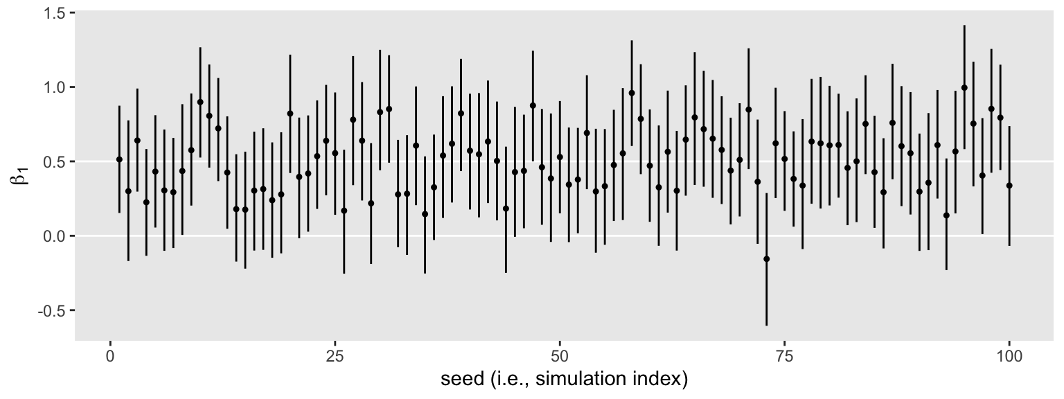
The horizontal lines show the idealized effect size (0.5) and the null hypothesis (0). Already, it’s apparent that most of our intervals indicate there’s more than a 95% probability the null hypothesis is not credible. Several do. Here’s how to quantify that.
parameters %>%
  filter(parameter == "treatment") %>%
  mutate(check = ifelse(Q2.5 > 0, 1, 0)) %>%
  summarise(power = mean(check))
## # A tibble: 1 × 1
##   power
##   <dbl>
## 1  0.67
With the second mutate() line, we used a logical statement within ifelse() to code all instances where the lower limit of the 95% interval (Q2.5) was greater than 0 as a 1, with the rest as 0. That left us with a vector of 1’s and 0’s, which we saved as check. In the summarise() line, we took the mean of that column, which returned our Bayesian power estimate.
That is, in 66 of our 100 simulations, an \(n = 50\) per group was enough to produce a 95% Bayesian credible interval that did not straddle 0.
I should probably point out that a 95% interval for which Q97.5 < 0 would have also been consistent with the alternative hypothesis of \(\mu_c \neq \mu_t\). However, I didn’t bother to work that option into the definition of our check variable because I knew from the outset that that would be a highly unlikely result. But if you’d like to work more rigor into your checks, by all means do.
And if you’ve gotten this far and have been following along with code of your own, congratulations! You did it! You’ve estimated the power of a Bayesian model with a given \(n\). Now let’s refine our approach.
Version 2: We might should be more careful with memory.
I really like it that our s object contains all our brm() fits. It makes it really handy to do global diagnostics like making sure our \(\widehat R\) values are all within a respectable range.
s %>%
  mutate(rhat = map(fit, rhat)) %>%
  unnest(rhat) %>%

  ggplot(aes(x = rhat)) +
  geom_histogram(bins = 20)
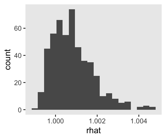
Man those \(\widehat R\) values look sweet. It’s great to have a workflow that lets you check them. But holding on to all those fits can take up a lot of memory. If the only thing you’re interested in are the parameter summaries, a better approach might be to do the model refitting and parameter extraction in one step. That way you only save the parameter summaries. Here’s how you might do that.
t3 <- Sys.time()

s2 <-
  tibble(seed = 1:n_sim) %>%
  mutate(d = map(seed, sim_d, n = 50)) %>%
  # here's the new part
  mutate(b1 = map2(d, seed, ~update(fit, newdata = .x, seed = .y) %>%
                     fixef() %>%
                     data.frame() %>%
                     rownames_to_column("parameter") %>%
                     filter(parameter == "treatment")))

t4 <- Sys.time()
Like before, this only about a minute.
t4 - t3
## Time difference of 1.156098 mins
As a point of comparison, here are the sizes of the results from our first approach to those from the second.
object.size(s)
## 87125520 bytes
object.size(s2)
## 503120 bytes
That’s a big difference. Hopefully you get the idea. With more complicated models and 10+ times the number of simulations, size will eventually matter.
Anyway, here are the results.
s2 %>%
  unnest(b1) %>%

  ggplot(aes(x = seed, y = Estimate, ymin = Q2.5, ymax = Q97.5)) +
  geom_hline(yintercept = c(0, .5), color = "white") +
  geom_pointrange(fatten = 1/2) +
  labs(x = "seed (i.e., simulation index)",
       y = expression(beta[1]))

Same parameter summaries, lower memory burden.
Version 3: Still talking about memory, we can be even stingier.
So far, both of our simulation attempts resulted in our saving the simulated data sets. It’s a really nice option if you ever want to go back and take a look at those simulated data. For example, you might want to inspect a random subset of the data simulations with box plots.
set.seed(1)

s2 %>%
  sample_n(12) %>%
  unnest(d) %>%

  ggplot(aes(x = group, y = y)) +
  geom_boxplot(aes(fill = group),
               alpha = 2/3, show.legend = F) +
  scale_fill_manual(values = c("grey25", "blue2")) +
  xlab(NULL) +
  facet_wrap(~ seed)
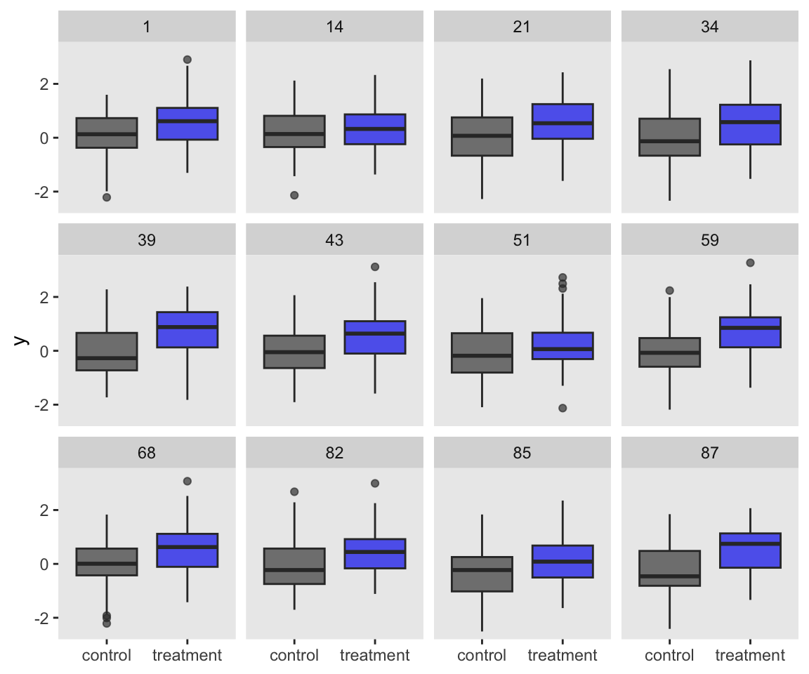
In this case, it’s no big deal if we keep the data around or not. The data sets are fairly small and we’re only simulating 100 of them. But in cases where the data are larger and you’re doing thousands of simulations, keeping the data could become a memory drain.
If you’re willing to forgo the luxury of inspecting your data simulations, it might make sense to run our power analysis in a way that avoids saving them. One way to do so would be to just wrap the data simulation and model fitting all in one function. We’ll call it sim_d_and_fit().
sim_d_and_fit <- function(seed, n) {

  mu_t <- .5
  mu_c <- 0

  set.seed(seed)

  d <-
    tibble(group     = rep(c("control", "treatment"), each = n)) %>%
    mutate(treatment = ifelse(group == "control", 0, 1),
           y         = ifelse(group == "control",
                              rnorm(n, mean = mu_c, sd = 1),
                              rnorm(n, mean = mu_t, sd = 1)))

  update(fit,
         newdata = d,
         seed = seed) %>%
    fixef() %>%
    data.frame() %>%
    rownames_to_column("parameter") %>%
    filter(parameter == "treatment")
}
Now iterate 100 times once more.
t5 <- Sys.time()

s3 <-
  tibble(seed = 1:n_sim) %>%
  mutate(b1 = map(seed, sim_d_and_fit, n = 50)) %>%
  unnest(b1)

t6 <- Sys.time()
That was pretty quick.
t6 - t5
## Time difference of 1.353221 mins
Here’s what it returned.
head(s3)
## # A tibble: 6 × 6
##    seed parameter Estimate Est.Error    Q2.5 Q97.5
##   <int> <chr>        <dbl>     <dbl>   <dbl> <dbl>
## 1     1 treatment    0.513     0.183  0.153  0.874
## 2     2 treatment    0.300     0.241 -0.170  0.776
## 3     3 treatment    0.640     0.174  0.297  0.990
## 4     4 treatment    0.225     0.183 -0.135  0.583
## 5     5 treatment    0.432     0.194  0.0552 0.810
## 6     6 treatment    0.305     0.209 -0.101  0.714
By wrapping our data simulation, model fitting, and parameter extraction steps all in one function, we simplified the output such that we’re no longer holding on to the data simulations or the brms fit objects. We just have the parameter summaries and the seed, making the product even smaller.
tibble(object = c("s", "s2", "s3")) %>%
  mutate(bytes = map_dbl(object, ~get(.) %>% object.size()))
## # A tibble: 3 × 2
##   object    bytes
##   <chr>     <dbl>
## 1 s      87125520
## 2 s2       503120
## 3 s3         5952
But the primary results are the same.
s3 %>%
  ggplot(aes(x = seed, y = Estimate, ymin = Q2.5, ymax = Q97.5)) +
  geom_hline(yintercept = c(0, .5), color = "white") +
  geom_pointrange(fatten = 1/2) +
  labs(x = "seed (i.e., simulation index)",
       y = expression(beta[1]))

We still get the same power estimate, too.
s3 %>%
  mutate(check = ifelse(Q2.5 > 0, 1, 0)) %>%
  summarise(power = mean(check))
## # A tibble: 1 × 1
##   power
##   <dbl>
## 1  0.67
Next steps
But my goal was to figure out what \(n\) will get me power of .8 or more!, you say. Fair enough. Try increasing n to 65 or something.
If that seems unsatisfying, welcome to the world of simulation. Since our Bayesian models are complicated, we don’t have the luxury of plugging a few values into some quick power formula. Just as simulation is an iterative process, determining on the right values to simulate over might well be an iterative process, too.
Wrap-up
Anyway, that’s the essence of the brms/tidyverse workflow for Bayesian power analysis. You follow these steps:
- Determine your primary data type.
- Determine your primary regression model and parameter(s) of interest.
- Pick defensible priors for all parameters–the kinds of priors you intend to use once you have the real data in hand.
- Select a sample size.
- Fit an initial model and save the fit object.
- Simulate some large number of data sets all following your prechosen form and use the
update()function to iteratively fit the models. - Extract the parameter(s) of interest.
- Summarize.
In addition, we played with a few approaches based on logistical concerns like memory. In the next post, part II, we’ll see how the precision-oriented approach to sample-size planning is a viable alternative to power focused on rejecting null hypotheses.
I had help.
Special thanks to Christopher Peters ( @statwonk) for the helpful edits and suggestions.
Session info
sessionInfo()
## R version 4.2.0 (2022-04-22)
## Platform: x86_64-apple-darwin17.0 (64-bit)
## Running under: macOS Big Sur/Monterey 10.16
##
## Matrix products: default
## BLAS:   /Library/Frameworks/R.framework/Versions/4.2/Resources/lib/libRblas.0.dylib
## LAPACK: /Library/Frameworks/R.framework/Versions/4.2/Resources/lib/libRlapack.dylib
##
## locale:
## [1] en_US.UTF-8/en_US.UTF-8/en_US.UTF-8/C/en_US.UTF-8/en_US.UTF-8
##
## attached base packages:
## [1] stats     graphics  grDevices utils     datasets  methods   base
##
## other attached packages:
##  [1] brms_2.18.0     Rcpp_1.0.9      forcats_0.5.1   stringr_1.4.1
##  [5] dplyr_1.0.10    purrr_0.3.4     readr_2.1.2     tidyr_1.2.1
##  [9] tibble_3.1.8    ggplot2_3.4.0   tidyverse_1.3.2
##
## loaded via a namespace (and not attached):
##   [1] readxl_1.4.1         backports_1.4.1      plyr_1.8.7
##   [4] igraph_1.3.4         splines_4.2.0        crosstalk_1.2.0
##   [7] TH.data_1.1-1        rstantools_2.2.0     inline_0.3.19
##  [10] digest_0.6.30        htmltools_0.5.3      fansi_1.0.3
##  [13] magrittr_2.0.3       checkmate_2.1.0      googlesheets4_1.0.1
##  [16] tzdb_0.3.0           modelr_0.1.8         RcppParallel_5.1.5
##  [19] matrixStats_0.62.0   xts_0.12.1           sandwich_3.0-2
##  [22] prettyunits_1.1.1    colorspace_2.0-3     rvest_1.0.2
##  [25] haven_2.5.1          xfun_0.35            callr_3.7.3
##  [28] crayon_1.5.2         jsonlite_1.8.3       lme4_1.1-31
##  [31] survival_3.4-0       zoo_1.8-10           glue_1.6.2
##  [34] gtable_0.3.1         gargle_1.2.0         emmeans_1.8.0
##  [37] distributional_0.3.1 pkgbuild_1.3.1       rstan_2.21.7
##  [40] abind_1.4-5          scales_1.2.1         mvtnorm_1.1-3
##  [43] DBI_1.1.3            miniUI_0.1.1.1       xtable_1.8-4
##  [46] stats4_4.2.0         StanHeaders_2.21.0-7 DT_0.24
##  [49] htmlwidgets_1.5.4    httr_1.4.4           threejs_0.3.3
##  [52] posterior_1.3.1      ellipsis_0.3.2       pkgconfig_2.0.3
##  [55] loo_2.5.1            farver_2.1.1         sass_0.4.2
##  [58] dbplyr_2.2.1         utf8_1.2.2           labeling_0.4.2
##  [61] tidyselect_1.1.2     rlang_1.0.6          reshape2_1.4.4
##  [64] later_1.3.0          munsell_0.5.0        cellranger_1.1.0
##  [67] tools_4.2.0          cachem_1.0.6         cli_3.4.1
##  [70] generics_0.1.3       broom_1.0.1          ggridges_0.5.3
##  [73] evaluate_0.18        fastmap_1.1.0        yaml_2.3.5
##  [76] processx_3.8.0       knitr_1.40           fs_1.5.2
##  [79] nlme_3.1-159         mime_0.12            projpred_2.2.1
##  [82] xml2_1.3.3           compiler_4.2.0       bayesplot_1.9.0
##  [85] shinythemes_1.2.0    rstudioapi_0.13      gamm4_0.2-6
##  [88] reprex_2.0.2         bslib_0.4.0          stringi_1.7.8
##  [91] highr_0.9            ps_1.7.2             blogdown_1.15
##  [94] Brobdingnag_1.2-8    lattice_0.20-45      Matrix_1.4-1
##  [97] nloptr_2.0.3         markdown_1.1         shinyjs_2.1.0
## [100] tensorA_0.36.2       vctrs_0.5.0          pillar_1.8.1
## [103] lifecycle_1.0.3      jquerylib_0.1.4      bridgesampling_1.1-2
## [106] estimability_1.4.1   httpuv_1.6.5         R6_2.5.1
## [109] bookdown_0.28        promises_1.2.0.1     gridExtra_2.3
## [112] codetools_0.2-18     boot_1.3-28          colourpicker_1.1.1
## [115] MASS_7.3-58.1        gtools_3.9.3         assertthat_0.2.1
## [118] withr_2.5.0          shinystan_2.6.0      multcomp_1.4-20
## [121] mgcv_1.8-40          parallel_4.2.0       hms_1.1.1
## [124] grid_4.2.0           coda_0.19-4          minqa_1.2.5
## [127] rmarkdown_2.16       googledrive_2.0.0    shiny_1.7.2
## [130] lubridate_1.8.0      base64enc_0.1-3      dygraphs_1.1.1.6
# for the hard-core scrollers:
# if you increase n to 65, the power becomes about .85
n_sim <- 100

t7 <- Sys.time()

s4 <-
  tibble(seed = 1:n_sim) %>%
  mutate(b1 = map(seed, sim_d_and_fit, n = 65))

t8 <- Sys.time()

t8 - t7

object.size(s4)

s4 %>%
  unnest(b1) %>%
  mutate(check = ifelse(Q2.5 > 0, 1, 0)) %>%
  summarise(power = mean(check))
References
Bürkner, P.-C. (2017). brms: An R package for Bayesian multilevel models using Stan. Journal of Statistical Software, 80(1), 1–28. https://doi.org/10.18637/jss.v080.i01
Bürkner, P.-C. (2018). Advanced Bayesian multilevel modeling with the R package brms. The R Journal, 10(1), 395–411. https://doi.org/10.32614/RJ-2018-017
Bürkner, P.-C. (2020). brms reference manual, Version 2.14.4. https://CRAN.R-project.org/package=brms/brms.pdf
Bürkner, P.-C. (2022). brms: Bayesian regression models using ’Stan’. https://CRAN.R-project.org/package=brms
Cohen, J. (1988). Statistical power analysis for the behavioral sciences. L. Erlbaum Associates. https://www.worldcat.org/title/statistical-power-analysis-for-the-behavioral-sciences/oclc/17877467
Gelman, A., Simpson, D., & Betancourt, M. (2017). The prior can often only be understood in the context of the likelihood. Entropy, 19(10, 10), 555. https://doi.org/10.3390/e19100555
Grolemund, G., & Wickham, H. (2017). R for data science. O’Reilly. https://r4ds.had.co.nz
Kruschke, J. K. (2015). Doing Bayesian data analysis: A tutorial with R, JAGS, and Stan. Academic Press. https://sites.google.com/site/doingbayesiandataanalysis/
Kurz, A. S. (2020). Doing Bayesian data analysis in brms and the tidyverse (version 0.3.0). https://bookdown.org/content/3686/
Kurz, A. S. (2020). Statistical rethinking with brms, Ggplot2, and the tidyverse: Second edition (version 0.1.1). https://bookdown.org/content/4857/
Kurz, A. S. (2020). Statistical rethinking with brms, ggplot2, and the tidyverse (version 1.2.0). https://doi.org/10.5281/zenodo.3693202
Maxwell, S. E., Kelley, K., & Rausch, J. R. (2008). Sample size planning for statistical power and accuracy in parameter estimation. Annual Review of Psychology, 59(1), 537–563. https://doi.org/10.1146/annurev.psych.59.103006.093735
McElreath, R. (2020). Statistical rethinking: A Bayesian course with examples in R and Stan (Second Edition). CRC Press. https://xcelab.net/rm/statistical-rethinking/
McElreath, R. (2015). Statistical rethinking: A Bayesian course with examples in R and Stan. CRC press. https://xcelab.net/rm/statistical-rethinking/
Peng, R. D. (2019). R programming for data science. https://bookdown.org/rdpeng/rprogdatascience/
R Core Team. (2022). R: A language and environment for statistical computing. R Foundation for Statistical Computing. https://www.R-project.org/
Stan Development Team. (2020, February 10). RStan: The R interface to Stan. https://cran.r-project.org/web/packages/rstan/vignettes/rstan.html
Stan Development Team. (2021a). Stan reference manual, Version 2.27. https://mc-stan.org/docs/2_27/reference-manual/
Stan Development Team. (2021b). Stan user’s guide, Version 2.26. https://mc-stan.org/docs/2_26/stan-users-guide/index.html
Wickham, H. (2020). The tidyverse style guide. https://style.tidyverse.org/
Wickham, H. (2022). tidyverse: Easily install and load the ’tidyverse’. https://CRAN.R-project.org/package=tidyverse
Wickham, H., Averick, M., Bryan, J., Chang, W., McGowan, L. D., François, R., Grolemund, G., Hayes, A., Henry, L., Hester, J., Kuhn, M., Pedersen, T. L., Miller, E., Bache, S. M., Müller, K., Ooms, J., Robinson, D., Seidel, D. P., Spinu, V., … Yutani, H. (2019). Welcome to the tidyverse. Journal of Open Source Software, 4(43), 1686. https://doi.org/10.21105/joss.01686
- Posted on:
- July 18, 2019
- Length:
- 27 minute read, 5624 words