Bayesian power analysis: Part II. Some might prefer precision to power

Version 1.1.0

Edited on April 21, 2021, to remove the broom::tidy() portion of the workflow.

tl;dr

When researchers decide on a sample size for an upcoming project, there are more things to consider than null-hypothesis-oriented power. Bayesian researchers might like to frame their concerns in terms of precision. Stick around to learn what and how.

Are Bayesians doomed to refer to \(H_0\) ¹ with sample-size planning?

If you read the first post in this series (click here for a refresher), you may have found yourself thinking: Sure, last time you avoided computing \(p\)-values with your 95% Bayesian credible intervals. But weren’t you still operating like a NHSTesting frequentist with all that \(H_0 / H_1\) talk?

Solid criticism. We didn’t even bother discussing all the type-I versus type-II error details. Yet they too were lurking in the background the way we just chose the typical .8 power benchmark. That’s not to say that a \(p\)-value oriented approach isn’t legitimate. It’s certainly congruent with what most reviewers would expect². But this all seems at odds with a model-oriented Bayesian approach, which is what I generally prefer. Happily, we have other options to explore.

Let’s just pick up where we left off.

Load our primary statistical packages.

library(tidyverse)
library(brms)

As a recap, here’s how we performed the last simulation-based Bayesian power analysis from part I. First, we simulated a single data set and fit an initial model.

# define the means
mu_c <- 0
mu_t <- 0.5

# determine the group size
n <- 50

# simulate the data
set.seed(1)
d <-
  tibble(group     = rep(c("control", "treatment"), each = n)) %>% 
  mutate(treatment = ifelse(group == "control", 0, 1),
         y         = ifelse(group == "control", 
                            rnorm(n, mean = mu_c, sd = 1),
                            rnorm(n, mean = mu_t, sd = 1)))
# fit the model
fit <-
  brm(data = d,
      family = gaussian,
      y ~ 0 + Intercept + treatment,
      prior = c(prior(normal(0, 2), class = b),
                prior(student_t(3, 1, 1), class = sigma)),
      seed = 1)

Next, we made a custom function that both simulated data sets and used the update() function to update that initial fit in order to avoid additional compilation time.

sim_d_and_fit <- function(seed, n) {
  
  mu_c <- 0
  mu_t <- 0.5
  
  set.seed(seed)
  
  d <-
    tibble(group = rep(c("control", "treatment"), each = n)) %>% 
    mutate(treatment = ifelse(group == "control", 0, 1),
           y         = ifelse(group == "control", 
                              rnorm(n, mean = mu_c, sd = 1),
                              rnorm(n, mean = mu_t, sd = 1)))
  
  update(fit,
         newdata = d, 
         seed = seed) %>% 
    fixef() %>% 
    data.frame() %>% 
    rownames_to_column("parameter") %>% 
    filter(parameter == "treatment")
}

Then we finally iterated over n_sim <- 100 times.

n_sim <- 100

s3 <-
  tibble(seed = 1:n_sim) %>% 
  mutate(b1 = map(seed, sim_d_and_fit, n = 50)) %>% 
  unnest(b1)

The results looked like so:

theme_set(theme_grey() +
            theme(panel.grid = element_blank()))

s3 %>% 
  ggplot(aes(x = seed, y = Estimate, ymin = Q2.5, ymax = Q97.5)) +
  geom_hline(yintercept = c(0, .5), color = "white") +
  geom_pointrange(fatten = 1/2) +
  labs(x = "seed (i.e., simulation index)",
       y = expression(beta[1]))

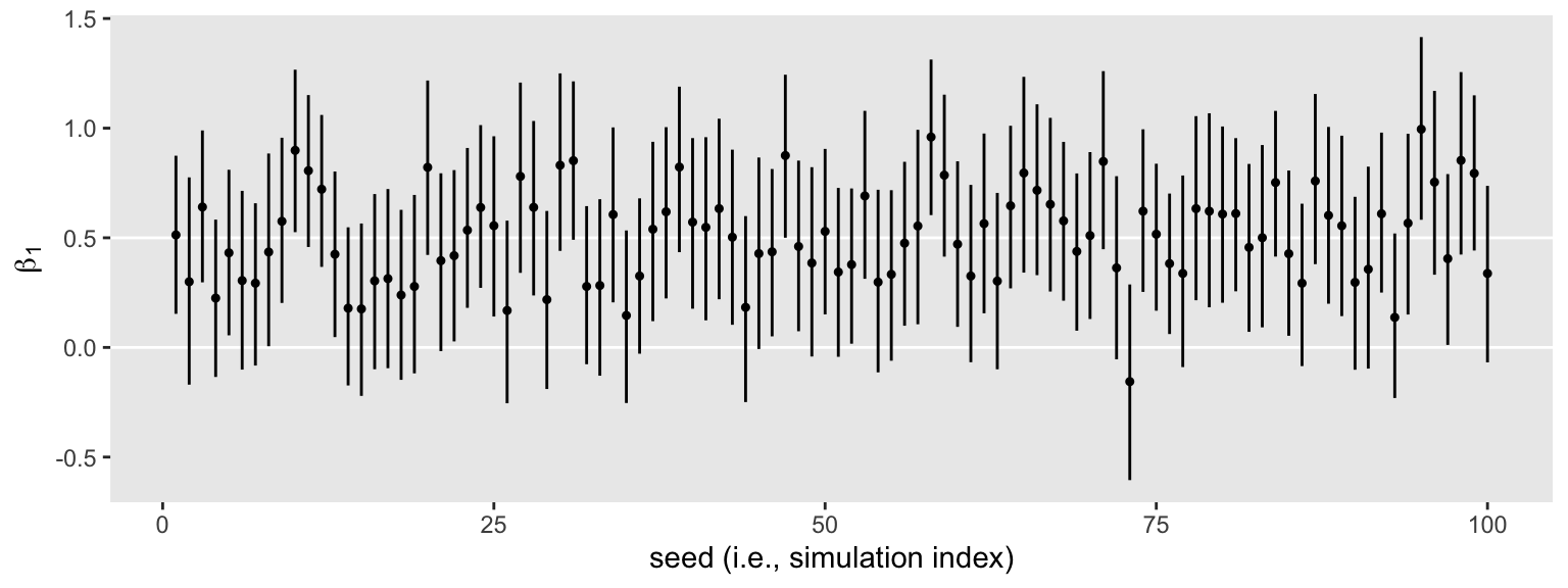
It’s time to build on the foundation.

We might evaluate “power” by widths.

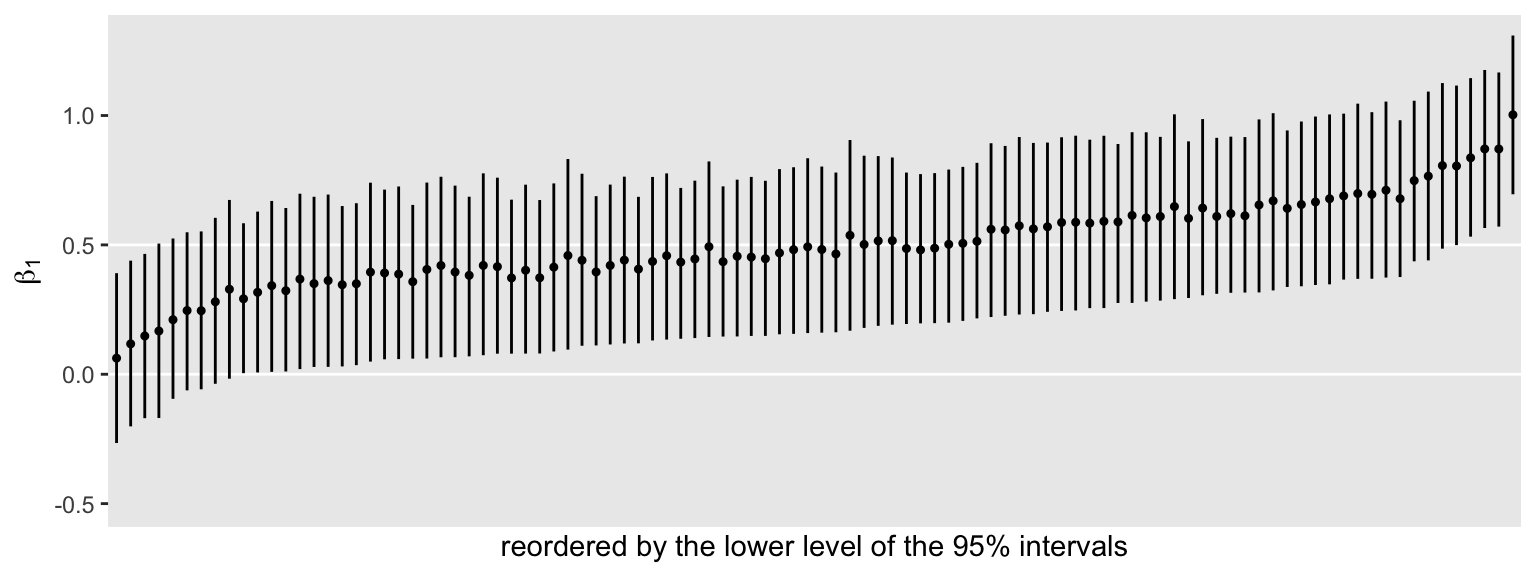
Instead of just ordering the point-ranges by their seed values, we might instead arrange them by the lower levels.

s3 %>%
  ggplot(aes(x = reorder(seed, Q2.5), y = Estimate, ymin = Q2.5, ymax = Q97.5)) +
  geom_hline(yintercept = c(0, .5), color = "white") +
  geom_pointrange(fatten = 1/2) +
  scale_x_discrete("reordered by the lower level of the 95% intervals", breaks = NULL) +
  ylab(expression(beta[1])) +
  coord_cartesian(ylim = c(-.5, 1.3))

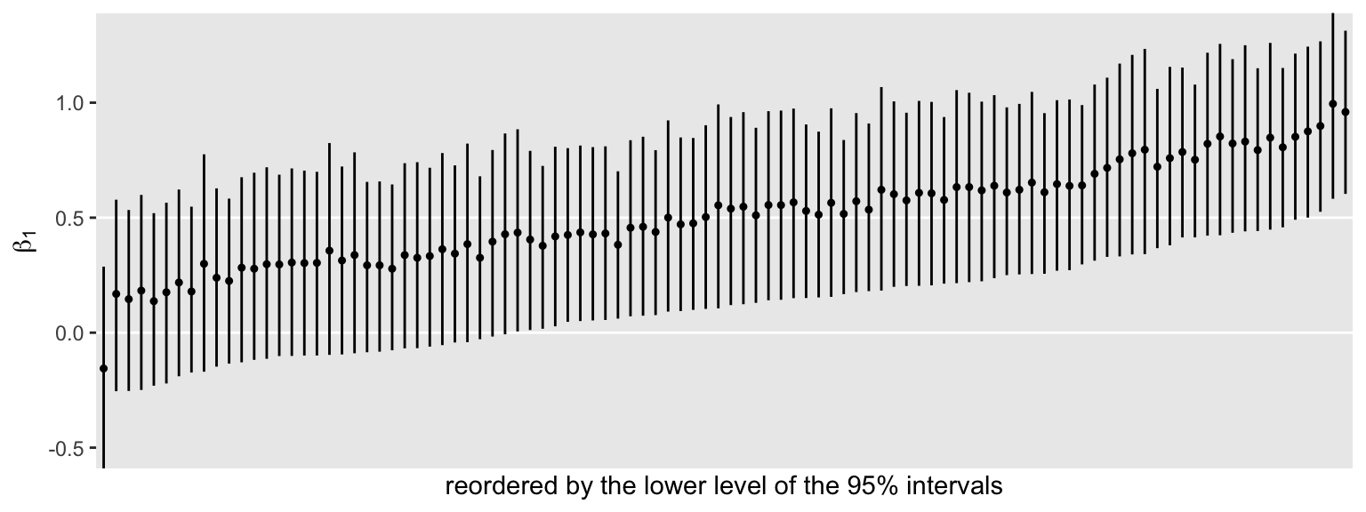
Notice how this arrangement highlights the differences in widths among the intervals. The wider the interval, the less precise the estimate. Some intervals were wider than others, but all tended to hover in a similar range. We might quantify those ranges by computing a width variable.

s3 <-
  s3 %>% 
  mutate(width = Q97.5 - Q2.5)

head(s3)

## # A tibble: 6 × 7
##    seed parameter Estimate Est.Error    Q2.5 Q97.5 width
##   <int> <chr>        <dbl>     <dbl>   <dbl> <dbl> <dbl>
## 1     1 treatment    0.513     0.183  0.153  0.874 0.721
## 2     2 treatment    0.300     0.241 -0.170  0.776 0.945
## 3     3 treatment    0.640     0.174  0.297  0.990 0.693
## 4     4 treatment    0.225     0.183 -0.135  0.583 0.717
## 5     5 treatment    0.432     0.194  0.0552 0.810 0.755
## 6     6 treatment    0.305     0.209 -0.101  0.714 0.815

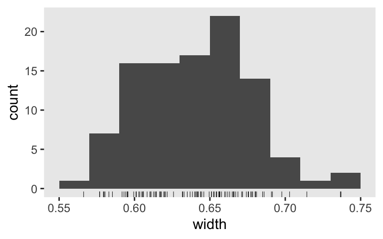
Here’s the width distribution.

s3 %>% 
  ggplot(aes(x = width)) +
  geom_histogram(binwidth = .01)

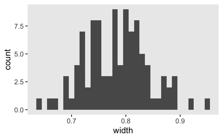
The widths of our 95% intervals range from 0.6 to 0.95, with the bulk sitting around 0.8. Let’s focus a bit and take a random sample from one of the simulation iterations.

set.seed(1)

s3 %>% 
  sample_n(1) %>% 
  mutate(seed = seed %>% as.character()) %>% 

  ggplot(aes(x = Estimate, xmin = Q2.5, xmax = Q97.5, y = seed)) +
  geom_vline(xintercept = c(0, .5), color = "white") +
  geom_pointrange() +
  labs(x = expression(beta[1]),
       y = "seed #") +
  xlim(0, 1)

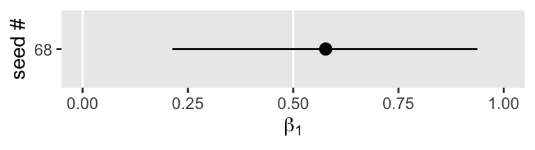
Though the posterior mean suggests the most probable value for \(\beta_1\) is about 0.6, the intervals suggest values from about 0.2 to almost 1 are within the 95% probability range. That’s a wide spread. Within psychology, a standardized mean difference of 0.2 would typically be considered small, whereas a difference of 1 would be large enough to raise a skeptical eyebrow or two.

So instead of focusing on rejecting a null hypothesis like \(\mu_\text{control} = \mu_\text{treatment}\), we might instead use our simulation skills to determine the sample size we need to have most of our 95% intervals come in at a certain level of precision. This has been termed the accuracy in parameter estimation [AIPE; Maxwell et al. ( 2008); see also Kruschke ( 2015)] approach to sample size planning.

Thinking in terms of AIPE, in terms of precision, let’s say we wanted widths of 0.7 or smaller. Here’s how we did with s3.

s3 %>% 
  mutate(check = ifelse(width < .7, 1, 0)) %>% 
  summarise(`width power` = mean(check))

## # A tibble: 1 × 1
##   `width power`
##           <dbl>
## 1          0.07

We did terrible. I’m not sure the term “width power” is even a thing. But hopefully you get the point. Our baby 100-iteration simulation suggests we have about a .08 probability of achieving 95% CI widths of 0.7 or smaller with \(n = 50\) per group. Though we’re pretty good at excluding zero, we don’t tend to do so with precision above that.

That last bit about excluding zero brings up an important point. Once we’re concerned about width size, about precision, the null hypothesis is no longer of direct relevance. And since we’re no longer wed to thinking in terms of the null hypothesis, there’s no real need to stick with a .8 threshold for evaluating width power (okay, I’ll stop using that term). Now if we wanted to stick with .8, we could. Though a little nonsensical, the .8 criterion would give our AIPE analyses a sense of familiarity with traditional power analyses, which some reviewers might appreciate. But in his text, Kruschke mentioned several other alternatives. One would be to set maximum value for our CI widths and simulate to find the \(n\) necessary so all our simulations pass that criterion. Another would follow Joseph, Wolfson, and du Berger ( 1995, 1995), who suggested we shoot for an \(n\) that produces widths that pass that criterion on average. Here’s how we did based on the average-width criterion.

s3 %>% 
  summarise(`average width` = mean(width))

## # A tibble: 1 × 1
##   `average width`
##             <dbl>
## 1           0.784

Close. Let’s see how increasing our sample size to 75 per group effects these metrics.

s4 <-
  tibble(seed = 1:n_sim) %>% 
  mutate(b1 = map(seed, sim_d_and_fit, n = 75)) %>% 
  unnest(b1) %>%
  mutate(width = Q97.5 - Q2.5)

Here’s what our new batch of 95% intervals looks like.

s4 %>% 
  ggplot(aes(x = reorder(seed, Q2.5), y = Estimate, ymin = Q2.5, ymax = Q97.5)) +
  geom_hline(yintercept = c(0, .5), color = "white") +
  geom_pointrange(fatten = 1/2) +
  scale_x_discrete("reordered by the lower level of the 95% intervals", breaks = NULL) +
  ylab(expression(beta[1])) +
  # this kept the scale on the y-axis the same as the simulation with n = 50
  coord_cartesian(ylim = c(-.5, 1.3))

Some of the intervals are still more precise than others, but they all now hover more tightly around their true data-generating value of 0.5. Here’s our updated “power” for producing interval widths smaller than 0.7.

s4 %>% 
  mutate(check = ifelse(width < .7, 1, 0)) %>% 
  summarise(`proportion below 0.7` = mean(check),
            `average width`        = mean(width))

## # A tibble: 1 × 2
##   `proportion below 0.7` `average width`
##                    <dbl>           <dbl>
## 1                   0.96           0.639

If we hold to the NHST-oriented .8 threshold, we did great and are even “overpowered”. We didn’t quite meet Kruschke’s strict limiting-worst-precision threshold, but we got close enough we’d have a good sense of what range of \(n\) values we might evaluate over next. As far as the mean-precision criterion, we did great by that one and even beat it.

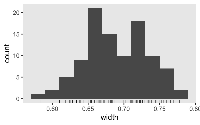
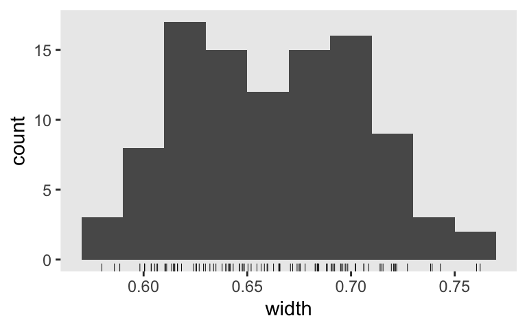
Here’s a look at how this batch of widths is distributed.

s4 %>% 
  ggplot(aes(x = width)) +
  geom_histogram(binwidth = .02) +
  geom_rug(size = 1/6)

## Warning: Using `size` aesthetic for lines was deprecated in ggplot2 3.4.0.
## ℹ Please use `linewidth` instead.

Let’s see if we can nail down the \(n\)s for our three AIPE criteria. Since we’re so close to fulfilling Kruschke’s limiting-worst-precision criterion, we’ll start there. I’m thinking \(n = 85\) should just about do it.

s5 <-
  tibble(seed = 1:n_sim) %>% 
  mutate(b1 = map(seed, sim_d_and_fit, n = 85)) %>% 
  unnest(b1) %>%
  mutate(width = Q97.5 - Q2.5)

Did we pass?

s5 %>% 
  mutate(check = ifelse(width < .7, 1, 0)) %>% 
  summarise(`proportion below 0.7` = mean(check))

## # A tibble: 1 × 1
##   `proportion below 0.7`
##                    <dbl>
## 1                      1

Success! We might look at how they’re distributed.

s5 %>% 
  ggplot(aes(x = width)) +
  geom_histogram(binwidth = .01) +
  geom_rug(size = 1/6)

A few of our simulated widths were approaching the 0.7 boundary. If we were to do a proper simulation with 1,000+ iterations, I’d worry one or two would creep over that boundary. So perhaps \(n = 90\) would be a better candidate for a large-scale simulation.

If we just wanted to meet the mean-precision criterion, we might look at something like \(n = 65\).

s6 <-
  tibble(seed = 1:n_sim) %>% 
  mutate(b1 = map(seed, sim_d_and_fit, n = 65)) %>% 
  unnest(b1) %>%
  mutate(width = Q97.5 - Q2.5)

Did we pass the mean-precision criterion?

s6 %>% 
  summarise(`average width` = mean(width))

## # A tibble: 1 × 1
##   `average width`
##             <dbl>
## 1           0.690

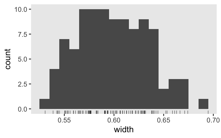
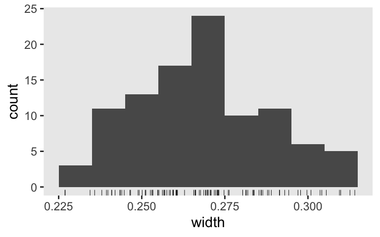
We got it! It looks like something like \(n = 65\) would be a good candidate for a larger-scale simulation. Here’s the distribution.

s6 %>% 
  ggplot(aes(x = width)) +
  geom_histogram(binwidth = .02) +
  geom_rug(size = 1/6)

For our final possible criterion, just get .8 of the widths below the threshold, we’ll want an \(n\) somewhere between 65 and 85. 70, perhaps?

s7 <-
  tibble(seed = 1:n_sim) %>% 
  mutate(b1 = map(seed, sim_d_and_fit, n = 70)) %>% 
  unnest(b1) %>%
  mutate(width = Q97.5 - Q2.5)

Did we pass the .8-threshold criterion?

s7 %>% 
  mutate(check = ifelse(width < .7, 1, 0)) %>% 
  summarise(`proportion below 0.7` = mean(check))

## # A tibble: 1 × 1
##   `proportion below 0.7`
##                    <dbl>
## 1                    0.8

Yep. Here’s the distribution.

s7 %>% 
  ggplot(aes(x = width)) +
  geom_histogram(binwidth = .02) +
  geom_rug(size = 1/6)

How are we defining our widths?

In frequentist analyses, we typically work with 95% confidence intervals because of their close connection to the conventional \(p < .05\) threshold. Another consequence of dropping our focus on rejecting \(H_0\) is that it no longer seems necessary to evaluate our posteriors with 95% intervals. And as it turns out, some Bayesians aren’t fans of the 95% interval. McElreath, for example, defiantly used 89% intervals in both editions of his ( 2020, 2015) text. In contrast, Gelman has blogged on his fondness for 50% intervals. Just for kicks, let’s follow Gelman’s lead and practice evaluating an \(n\) based on 50% intervals. This will require us to update our sim_d_and_fit() function to allow us to change the probs setting in the fixef() function.

sim_d_and_fit <- function(seed, n, probs = c(.25, .75)) {
  
  mu_c <- 0
  mu_t <- 0.5
  
  set.seed(seed)
  
  d <-
    tibble(group = rep(c("control", "treatment"), each = n)) %>% 
    mutate(treatment = ifelse(group == "control", 0, 1),
           y         = ifelse(group == "control", 
                              rnorm(n, mean = mu_c, sd = 1),
                              rnorm(n, mean = mu_t, sd = 1)))
  
  update(fit,
         newdata = d, 
         seed = seed) %>% 
    fixef(probs = probs) %>% 
    data.frame() %>% 
    rownames_to_column("parameter") %>% 
    filter(parameter == "treatment")
}

To make things simple, we just set the default probs settings to return 50% intervals. Now we simulate to examine those 50% intervals. We’ll start with the original \(n = 50\).

n_sim <- 100

s8 <-
  tibble(seed = 1:n_sim) %>% 
  mutate(b1 = map(seed, sim_d_and_fit, n = 50)) %>% 
  unnest(b1) %>% 
  # notice the change to this line of code
  mutate(width = Q75 - Q25)

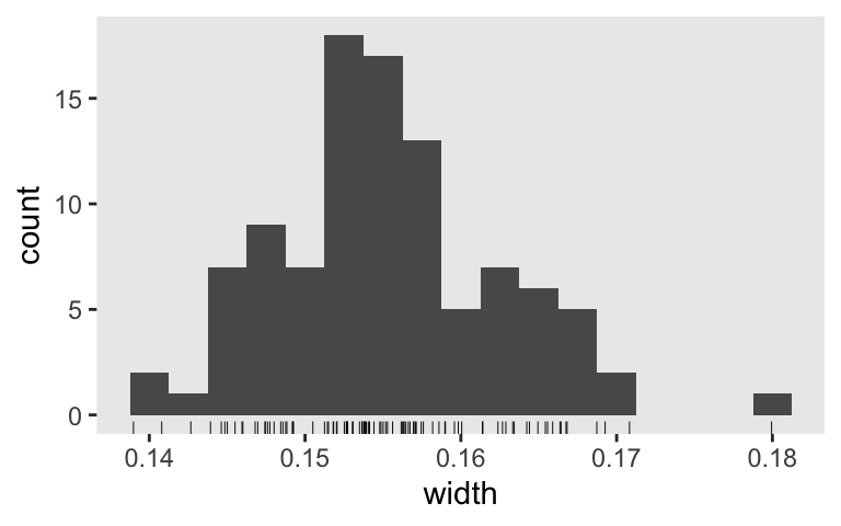
Here is the distribution of our 50% interval widths.

s8 %>% 
  mutate(width = Q75 - Q25) %>% 
  
  ggplot(aes(x = width)) +
  geom_histogram(binwidth = .01) +
  geom_rug(size = 1/6)

Since we’ve gone from 95% to 50% intervals, it should be no surprise that their widths are narrower. Accordingly, we should evaluate then with a higher standard. Perhaps it’s more reasonable to ask for an average width of 0.1. Let’s see how close \(n = 150\) gets us.

s9 <-
  tibble(seed = 1:n_sim) %>% 
  mutate(b1 = map(seed, sim_d_and_fit, n = 150)) %>% 
  unnest(b1) %>% 
  mutate(width = Q75 - Q25)

Look at the distribution.

s9 %>% 
  ggplot(aes(x = width)) +
  geom_histogram(binwidth = .0025) +
  geom_rug(size = 1/6)

Nope, we’re not there yet. Perhaps \(n = 200\) or \(250\) is the ticket. This is an iterative process. Anyway, once we’re talking that AIPE/precision/interval-width talk, we can get all kinds of creative with which intervals we’re even interested in. As far as I can tell, the topic is wide open for fights and collaborations between statisticians, methodologists, and substantive researchers to find sensible ways forward.

Maybe you should write a dissertation on it.

Regardless, get ready for part III where we’ll liberate ourselves from the tyranny of the Gauss.

Session info

sessionInfo()

## R version 4.2.0 (2022-04-22)
## Platform: x86_64-apple-darwin17.0 (64-bit)
## Running under: macOS Big Sur/Monterey 10.16
## 
## Matrix products: default
## BLAS:   /Library/Frameworks/R.framework/Versions/4.2/Resources/lib/libRblas.0.dylib
## LAPACK: /Library/Frameworks/R.framework/Versions/4.2/Resources/lib/libRlapack.dylib
## 
## locale:
## [1] en_US.UTF-8/en_US.UTF-8/en_US.UTF-8/C/en_US.UTF-8/en_US.UTF-8
## 
## attached base packages:
## [1] stats     graphics  grDevices utils     datasets  methods   base     
## 
## other attached packages:
##  [1] brms_2.18.0     Rcpp_1.0.9      forcats_0.5.1   stringr_1.4.1  
##  [5] dplyr_1.0.10    purrr_0.3.4     readr_2.1.2     tidyr_1.2.1    
##  [9] tibble_3.1.8    ggplot2_3.4.0   tidyverse_1.3.2
## 
## loaded via a namespace (and not attached):
##   [1] readxl_1.4.1         backports_1.4.1      plyr_1.8.7          
##   [4] igraph_1.3.4         splines_4.2.0        crosstalk_1.2.0     
##   [7] TH.data_1.1-1        rstantools_2.2.0     inline_0.3.19       
##  [10] digest_0.6.30        htmltools_0.5.3      fansi_1.0.3         
##  [13] magrittr_2.0.3       checkmate_2.1.0      googlesheets4_1.0.1 
##  [16] tzdb_0.3.0           modelr_0.1.8         RcppParallel_5.1.5  
##  [19] matrixStats_0.62.0   xts_0.12.1           sandwich_3.0-2      
##  [22] prettyunits_1.1.1    colorspace_2.0-3     rvest_1.0.2         
##  [25] haven_2.5.1          xfun_0.35            callr_3.7.3         
##  [28] crayon_1.5.2         jsonlite_1.8.3       lme4_1.1-31         
##  [31] survival_3.4-0       zoo_1.8-10           glue_1.6.2          
##  [34] gtable_0.3.1         gargle_1.2.0         emmeans_1.8.0       
##  [37] distributional_0.3.1 pkgbuild_1.3.1       rstan_2.21.7        
##  [40] abind_1.4-5          scales_1.2.1         mvtnorm_1.1-3       
##  [43] DBI_1.1.3            miniUI_0.1.1.1       xtable_1.8-4        
##  [46] stats4_4.2.0         StanHeaders_2.21.0-7 DT_0.24             
##  [49] htmlwidgets_1.5.4    httr_1.4.4           threejs_0.3.3       
##  [52] posterior_1.3.1      ellipsis_0.3.2       pkgconfig_2.0.3     
##  [55] loo_2.5.1            farver_2.1.1         sass_0.4.2          
##  [58] dbplyr_2.2.1         utf8_1.2.2           labeling_0.4.2      
##  [61] tidyselect_1.1.2     rlang_1.0.6          reshape2_1.4.4      
##  [64] later_1.3.0          munsell_0.5.0        cellranger_1.1.0    
##  [67] tools_4.2.0          cachem_1.0.6         cli_3.4.1           
##  [70] generics_0.1.3       broom_1.0.1          ggridges_0.5.3      
##  [73] evaluate_0.18        fastmap_1.1.0        yaml_2.3.5          
##  [76] processx_3.8.0       knitr_1.40           fs_1.5.2            
##  [79] nlme_3.1-159         mime_0.12            projpred_2.2.1      
##  [82] xml2_1.3.3           compiler_4.2.0       bayesplot_1.9.0     
##  [85] shinythemes_1.2.0    rstudioapi_0.13      gamm4_0.2-6         
##  [88] reprex_2.0.2         bslib_0.4.0          stringi_1.7.8       
##  [91] highr_0.9            ps_1.7.2             blogdown_1.15       
##  [94] Brobdingnag_1.2-8    lattice_0.20-45      Matrix_1.4-1        
##  [97] nloptr_2.0.3         markdown_1.1         shinyjs_2.1.0       
## [100] tensorA_0.36.2       vctrs_0.5.0          pillar_1.8.1        
## [103] lifecycle_1.0.3      jquerylib_0.1.4      bridgesampling_1.1-2
## [106] estimability_1.4.1   httpuv_1.6.5         R6_2.5.1            
## [109] bookdown_0.28        promises_1.2.0.1     gridExtra_2.3       
## [112] codetools_0.2-18     boot_1.3-28          colourpicker_1.1.1  
## [115] MASS_7.3-58.1        gtools_3.9.3         assertthat_0.2.1    
## [118] withr_2.5.0          shinystan_2.6.0      multcomp_1.4-20     
## [121] mgcv_1.8-40          parallel_4.2.0       hms_1.1.1           
## [124] grid_4.2.0           minqa_1.2.5          coda_0.19-4         
## [127] rmarkdown_2.16       googledrive_2.0.0    shiny_1.7.2         
## [130] lubridate_1.8.0      base64enc_0.1-3      dygraphs_1.1.1.6

References

Joseph, L., Wolfson, D. B., & Berger, R. D. (1995). Sample size calculations for binomial proportions via highest posterior density intervals. Journal of the Royal Statistical Society: Series D (The Statistician), 44(2), 143–154. https://doi.org/10.2307/2348439
Joseph, L., Wolfson, D. B., & Berger, R. D. (1995). Some comments on Bayesian sample size determination. Journal of the Royal Statistical Society: Series D (The Statistician), 44(2), 167–171. https://doi.org/10.2307/2348442
Kruschke, J. K. (2015). Doing Bayesian data analysis: A tutorial with R, JAGS, and Stan. Academic Press. https://sites.google.com/site/doingbayesiandataanalysis/
Maxwell, S. E., Kelley, K., & Rausch, J. R. (2008). Sample size planning for statistical power and accuracy in parameter estimation. Annual Review of Psychology, 59(1), 537–563. https://doi.org/10.1146/annurev.psych.59.103006.093735
McElreath, R. (2020). Statistical rethinking: A Bayesian course with examples in R and Stan (Second Edition). CRC Press. https://xcelab.net/rm/statistical-rethinking/
McElreath, R. (2015). Statistical rethinking: A Bayesian course with examples in R and Stan. CRC press. https://xcelab.net/rm/statistical-rethinking/
Morey, R. D., & Rouder, J. N. (2011). Bayes factor approaches for testing interval null hypotheses. Psychological Methods, 16(4), 406–419. https://doi.org/10.1037/a0024377
Rouder, J. N., Speckman, P. L., Sun, D., Morey, R. D., & Iverson, G. (2009). Bayesian t tests for accepting and rejecting the null hypothesis. Psychonomic Bulletin & Review, 16(2), 225–237. https://doi.org/10.3758/PBR.16.2.225
Wasserstein, R. L., Schirm, A. L., & Lazar, N. A. (2019). Moving to a World Beyond “p $<$ 0.05.” The American Statistician, 73, 1–19. https://doi.org/10.1080/00031305.2019.1583913
-
To be clear, one can consider the null hypothesis within the Bayesian paradigm. I don’t tend to take this approach, but it’d be unfair not to at least mention some resources. Kurschke covered the topic in chapters 11 and 12 in his ( 2015) text, Doing Bayesian data analysis: A tutorial with R, JAGS, and Stan. You might also check out Rouder et al. ( 2009), Bayesian t tests for accepting and rejecting the null hypothesis, or Morey & Rouder ( 2011), Bayes factor approaches for testing interval null hypotheses. ↩︎
For a contemporary discussion of the uses and misuses of
\(p\)-values, see Wasserstein et al. ( 2019) and the other articles contained in that special issue of The American Statistician. ↩︎
- Posted on:
- July 24, 2019
- Length:
- 15 minute read, 2990 words