Make ICC plots for your brms IRT models
By A. Solomon Kurz
June 29, 2021
Version 1.1.0
Edited on December 12, 2022, to use the new as_draws_df() workflow.
Context
Someone recently posted a thread on the Stan forums asking how one might make item-characteristic curve (ICC) and item-information curve (IIC) plots for an item-response theory (IRT) model fit with brms. People were slow to provide answers and I came up disappointingly empty handed after a quick web search. The purpose of this blog post is to show how one might make ICC and IIC plots for brms IRT models using general-purpose data wrangling steps.
I make assumptions.
This tutorial is for those with a passing familiarity with the following:
-
You’ll want to be familiar with the brms package ( Bürkner, 2017, 2018, 2022). In addition to the references I just cited, you can find several helpful vignettes at https://github.com/paul-buerkner/brms. I’ve also written a few ebooks highlighting brms, which you can find at https://solomonkurz.netlify.app/bookdown/.
-
You’ll want to be familiar with Bayesian multilevel regression. In addition to the resources, above, I recommend either edition of McElreath’s introductory text ( 2020, 2015) or Kruschke’s ( 2015) introductory text.
-
You’ll want to be familiar with IRT. The framework in this blog comes most directly from Bürkner’s ( 2020) preprint. Though I’m not in a position to vouch for them myself, I’ve had people recommend the texts by Crocker & Algina ( 2006); De Ayala ( 2008); Reckase ( 2009); Bonifay ( 2019)1; and Albano ( 2020).
-
All code is in R ( R Core Team, 2022), with healthy doses of the tidyverse ( Wickham et al., 2019; Wickham, 2022). Probably the best place to learn about the tidyverse-style of coding, as well as an introduction to R, is Grolemund and Wickham’s ( 2017) freely-available online text, R for data science.
Load the primary R packages.
library(tidyverse)
library(brms)
Data
The data for this post come from the preprint by Loram et al. ( 2019), who generously shared their data and code on GitHub and the Open Science Framework. In their paper, they used IRT to make a self-report measure of climate change denial. After pruning their initial item set, Loram and colleagues settled on eight binary items for their measure. Here we load the data for those items2.
load("data/ccdrefined02.rda")

ccdrefined02 %>%
  glimpse()
## Rows: 206
## Columns: 8
## $ ccd05 <dbl> 0, 0, 0, 0, 0, 0, 0, 0, 0, 1, 0, 0, 0, 0, 0, 0, 0, 0, 0, 0, 0, 0, 0, 0, 0, 1, 0, 0, 1, 0, 0, 0…
## $ ccd18 <dbl> 0, 0, 0, 0, 0, 0, 1, 0, 0, 0, 0, 0, 0, 1, 0, 0, 0, 0, 0, 0, 0, 0, 1, 0, 0, 1, 0, 0, 0, 0, 0, 0…
## $ ccd11 <dbl> 1, 0, 1, 0, 0, 0, 0, 0, 0, 1, 0, 0, 0, 1, 0, 0, 0, 0, 0, 0, 0, 0, 0, 0, 1, 0, 0, 0, 1, 0, 0, 0…
## $ ccd13 <dbl> 1, 0, 0, 0, 0, 0, 0, 0, 0, 0, 0, 0, 0, 1, 0, 0, 0, 0, 0, 0, 0, 0, 1, 0, 0, 0, 0, 0, 1, 0, 1, 0…
## $ ccd08 <dbl> 0, 0, 1, 0, 0, 0, 1, 0, 0, 0, 0, 0, 0, 0, 1, 0, 0, 0, 0, 0, 0, 0, 1, 0, 1, 0, 0, 1, 0, 0, 1, 0…
## $ ccd06 <dbl> 1, 0, 1, 0, 0, 0, 1, 0, 0, 1, 0, 0, 0, 0, 1, 0, 0, 0, 0, 0, 0, 0, 0, 0, 1, 0, 0, 1, 1, 0, 1, 0…
## $ ccd09 <dbl> 1, 0, 1, 0, 0, 0, 1, 0, 0, 1, 0, 0, 0, 0, 0, 0, 0, 0, 0, 0, 0, 0, 0, 0, 1, 1, 0, 1, 1, 0, 1, 0…
## $ ccd16 <dbl> 1, 0, 1, 0, 0, 0, 0, 0, 1, 1, 0, 0, 0, 0, 1, 0, 0, 0, 0, 0, 0, 0, 0, 0, 1, 1, 0, 0, 1, 0, 1, 0…
If you walk through the code in Loram and colleagues’
2018_Loram_CC_IRT.R file, you’ll see where this version of the data comes from. For our purposes, we’ll want to make an explicit participant number column and then convert the data to the long format.
dat_long <- ccdrefined02 %>%
  mutate(id = 1:n()) %>%
  pivot_longer(-id, names_to = "item", values_to = "y") %>%
  mutate(item = str_remove(item, "ccd"))

# what did we do?
head(dat_long)
## # A tibble: 6 × 3
##      id item      y
##   <int> <chr> <dbl>
## 1     1 05        0
## 2     1 18        0
## 3     1 11        1
## 4     1 13        1
## 5     1 08        0
## 6     1 06        1
Now responses (y) are nested within participants (id) and items (item).
IRT
In his -Bürkner (
2020) preprint, Bürkner outlined the framework for the multilevel Bayesian approach to IRT, as implemented in brms. In short, IRT allows one to decompose the information from assessment measures into person parameters \((\theta)\) and item parameters \((\xi)\). The IRT framework offers a large variety of model types. In this post, we’ll focus on the widely-used 1PL and 2PL models. First, we’ll briefly introduce them within the context of Bürkner’s multilevel Bayesian approach. Then we’ll fit those models to the dat_long data. Finally, we’ll show how to explore those models using ICC and IIC plots.
What is the 1PL?
With a set of binary data \(y_{pi}\), which vary across \(P\) persons and \(I\) items, we can express the simple one-parameter logistic (1PL) model as
$$
\begin{align*} y_{pi} & \sim \operatorname{Bernoulli}(p_{pi}) \\ \operatorname{logit}(p_{pi}) & = \theta_p + \xi_i, \end{align*}
$$
where the \(p_{pi}\) parameter from the Bernoulli distribution indicates the probability of 1 for the \(p\text{th}\) person on the \(i\text{th}\) item. To constrain the model predictions to within the \([0, 1]\) probability space, we use the logit link. Note that with this parameterization, the linear model itself is just the additive sum of the person parameter \(\theta_p\) and item parameter \(\xi_i\).
Within our multilevel Bayesian framework, we will expand this a bit to
$$
\begin{align*} y_{pi} & \sim \operatorname{Bernoulli}(p_{pi}) \\ \operatorname{logit}(p_{pi}) & = \beta_0 + \theta_p + \xi_i \\ \theta_p & \sim \operatorname{Normal}(0, \sigma_\theta) \\ \xi_i & \sim \operatorname{Normal}(0, \sigma_\xi), \end{align*}
$$
where the new parameter \(\beta_0\) is the grand mean. Now our \(\theta_p\) and \(\xi_i\) parameters are expressed as deviations around the grand mean \(\beta_0\). As is typical within the multilevel framework, we model these deviations as normally distributed with means set to zero and standard deviations ($\sigma_\theta$ and \(\sigma_\xi\)) estimated from the data3.
To finish off our multilevel Bayesian version the 1PL, we just need to add in our priors. In this blog post, we’ll follow the weakly-regularizing approach and set
$$
\begin{align*} \beta_0 & \sim \operatorname{Normal}(0, 1.5) \\ \sigma_\theta & \sim \operatorname{Student-t}^+(10, 0, 1) \\ \sigma_\xi & \sim \operatorname{Student-t}^+(10, 0, 1), \end{align*}
$$
where the \(+\) superscripts indicate the Student-$t$ priors for the \(\sigma\) parameters are restricted to non-negative values.
How about the 2PL?
We can express the two-parameter logistic (2PL) model as
$$
\begin{align*} y_{pi} & \sim \operatorname{Bernoulli}(p_{pi}) \\ \operatorname{logit}(p_{pi}) & = \alpha_i \theta_p + \alpha_i \xi_i \\ & = \alpha_i(\theta_p + \xi_i), \end{align*}
$$
where the \(\theta_p\) and \(\xi_i\) parameters are now both multiplied by the discrimination parameter \(\alpha_i\). The \(i\) subscript indicates the discrimination parameter varies across the items, but not across persons. We should note that because we are now multiplying parameters, this makes the 2PL a non-liner model. Within our multilevel Bayesian framework, we might express the 2PL as
$$
\begin{align*} y_{pi} & \sim \operatorname{Bernoulli}(p_{pi}) \\ \operatorname{logit}(p_{pi}) & = \alpha (\beta_0 + \theta_p + \xi_i) \\ \alpha & = \beta_1 + \alpha_i \\ \theta_p & \sim \operatorname{Normal}(0, \sigma_\theta) \\ \begin{bmatrix} \alpha_i \\ \xi_i \end{bmatrix} & \sim \operatorname{MVNormal}(\mathbf 0, \mathbf \Sigma) \\ \Sigma & = \mathbf{SRS} \\ \mathbf S & = \begin{bmatrix} \sigma_\alpha & 0 \\ 0 & \sigma_\xi \end{bmatrix} \\ \mathbf R & = \begin{bmatrix} 1 & \rho \\ \rho & 1 \end{bmatrix} , \end{align*}
$$
where the \(\alpha\) term is multiplied by \(\beta_0\), in addition to the \(\theta_p\) and \(\xi_i\) parameters. But note that \(\alpha\) is itself a composite of its own grand mean \(\beta_1\) and the item-level deviations around it, \(\alpha_i\). Since both \(\alpha\) and \(\xi\) vary across items, they are modeled as multivariate normal, with a mean vector of zeros and variance/covariance matrix \(\mathbf \Sigma\). As is typical with brms, we will decompose \(\mathbf \Sigma\) into a diagonal matrix of standard deviations \((\mathbf S)\) and a correlation matrix \((\mathbf R)\).
As Bürkner (
2020) discussed in Section 5, this particular model might have identification problems without strong priors. The issue is “a switch in the sign of \([\alpha]\) can be corrected for by a switch in the sign of \([(\beta_0 + \theta_p + \xi_i)]\) without a change in the overall likelihood.” One solution, then, would be to constrain \(\alpha\) to be positive. We can do that with
$$
\begin{align*} y_{pi} & \sim \operatorname{Bernoulli}(p_{pi}) \\ \operatorname{logit}(p_{pi}) & = \color{#8b0000}{ \exp(\log \alpha) } \color{#000000}{\times (\beta_0 + \theta_p + \xi_i)} \\ \color{#8b0000}{\log \alpha} & = \beta_1 + \alpha_i \\ \theta_p & \sim \operatorname{Normal}(0, \sigma_\theta) \\ \begin{bmatrix} \alpha_i \\ \xi_i \end{bmatrix} & \sim \operatorname{MVNormal}(\mathbf 0, \mathbf \Sigma) \\ \Sigma & = \mathbf{SRS} \\ \mathbf S & = \begin{bmatrix} \sigma_\alpha & 0 \\ 0 & \sigma_\xi \end{bmatrix} \\ \mathbf R & = \begin{bmatrix} 1 & \rho \\ \rho & 1 \end{bmatrix}, \end{align*}
$$
wherein we are now modeling \(\alpha\) on the log scale and then exponentiating \(\log \alpha\) within the linear formula for \(\operatorname{logit}(p_{pi})\). Continuing on with our weakly-regularizing approach, we will express our priors for this model as
$$
\begin{align*} \beta_0 & \sim \operatorname{Normal}(0, 1.5) \\ \beta_1 & \sim \operatorname{Normal}(0, 1) \\ \sigma_\theta & \sim \operatorname{Student-t}^+(10, 0, 1) \\ \sigma_\alpha & \sim \operatorname{Student-t}^+(10, 0, 1) \\ \sigma_\xi & \sim \operatorname{Student-t}^+(10, 0, 1) \\ \mathbf R & \sim \operatorname{LKJ}(2), \end{align*}
$$
where LKJ is the Lewandowski, Kurowicka, and Joe prior for correlation matrices (
Lewandowski et al., 2009). With \(\eta = 2\), the LKJ weakly regularizes the correlations away from extreme values4.
Fire up brms.
With brms::brm(), we can fit our 1PL model with conventional multilevel syntax.
irt1 <- brm(
  data = dat_long,
  family = brmsfamily("bernoulli", "logit"),
  y ~ 1 + (1 | item) + (1 | id),
  prior = c(prior(normal(0, 1.5), class = Intercept),
            prior(student_t(10, 0, 1), class = sd)),
  cores = 4, seed = 1
)
Our non-linear 2PL model, however, will require the brms non-linear syntax ( Bürkner, 2021). Here we’ll follow the same basic configuration Bürkner used in his ( 2020) IRT preprint.
irt2 <- brm(
  data = dat_long,
  family = brmsfamily("bernoulli", "logit"),
  bf(
    y ~ exp(logalpha) * eta,
    eta ~ 1 + (1 |i| item) + (1 | id),
    logalpha ~ 1 + (1 |i| item),
    nl = TRUE
  ),
  prior = c(prior(normal(0, 1.5), class = b, nlpar = eta),
            prior(normal(0, 1), class = b, nlpar = logalpha),
            prior(student_t(10, 0, 1), class = sd, nlpar = eta),
            prior(student_t(10, 0, 1), class = sd, nlpar = logalpha),
            prior(lkj(2), class = cor)),
  cores = 4, seed = 1,
  control = list(adapt_delta = .99)
)
Note that for irt2, we had to adjust the adapt_delta settings to stave off a few divergent transitions. Anyway, here are the parameter summaries for the models.
print(irt1)
##  Family: bernoulli
##   Links: mu = logit
## Formula: y ~ 1 + (1 | item) + (1 | id)
##    Data: dat_long (Number of observations: 1648)
##   Draws: 4 chains, each with iter = 2000; warmup = 1000; thin = 1;
##          total post-warmup draws = 4000
##
## Group-Level Effects:
## ~id (Number of levels: 206)
##               Estimate Est.Error l-95% CI u-95% CI Rhat Bulk_ESS Tail_ESS
## sd(Intercept)     3.81      0.38     3.12     4.61 1.01     1129     2107
##
## ~item (Number of levels: 8)
##               Estimate Est.Error l-95% CI u-95% CI Rhat Bulk_ESS Tail_ESS
## sd(Intercept)     0.96      0.29     0.55     1.67 1.00     1814     2835
##
## Population-Level Effects:
##           Estimate Est.Error l-95% CI u-95% CI Rhat Bulk_ESS Tail_ESS
## Intercept    -2.88      0.47    -3.82    -1.94 1.00     1309     2040
##
## Draws were sampled using sampling(NUTS). For each parameter, Bulk_ESS
## and Tail_ESS are effective sample size measures, and Rhat is the potential
## scale reduction factor on split chains (at convergence, Rhat = 1).
print(irt2)
##  Family: bernoulli
##   Links: mu = logit
## Formula: y ~ exp(logalpha) * eta
##          eta ~ 1 + (1 | i | item) + (1 | id)
##          logalpha ~ 1 + (1 | i | item)
##    Data: dat_long (Number of observations: 1648)
##   Draws: 4 chains, each with iter = 2000; warmup = 1000; thin = 1;
##          total post-warmup draws = 4000
##
## Group-Level Effects:
## ~id (Number of levels: 206)
##                   Estimate Est.Error l-95% CI u-95% CI Rhat Bulk_ESS Tail_ESS
## sd(eta_Intercept)     1.78      0.69     0.68     3.39 1.00     1933     2321
##
## ~item (Number of levels: 8)
##                                       Estimate Est.Error l-95% CI u-95% CI Rhat Bulk_ESS Tail_ESS
## sd(eta_Intercept)                         0.50      0.25     0.16     1.16 1.00     1521     2181
## sd(logalpha_Intercept)                    0.36      0.16     0.13     0.74 1.00     1543     2075
## cor(eta_Intercept,logalpha_Intercept)     0.44      0.31    -0.26     0.90 1.00     2847     2922
##
## Population-Level Effects:
##                    Estimate Est.Error l-95% CI u-95% CI Rhat Bulk_ESS Tail_ESS
## eta_Intercept         -1.41      0.57    -2.71    -0.51 1.00     1701     2140
## logalpha_Intercept     0.91      0.42     0.16     1.82 1.00     1944     2282
##
## Draws were sampled using sampling(NUTS). For each parameter, Bulk_ESS
## and Tail_ESS are effective sample size measures, and Rhat is the potential
## scale reduction factor on split chains (at convergence, Rhat = 1).
I’m not going to bother interpreting these results because, well, this isn’t a full-blown IRT tutorial. For our purposes, we’ll just note that the \(\widehat R\) and effective sample size values all look good and nothing seems off with the parameter summaries. They’re not shown here, but the trace plots look good, too. We’re on good footing to explore the models with our ICC and IIC plots.
ICCs.
For IRT models of binary items, item-characteristic curves (ICCs) show the expected relation between one’s underlying “ability” and the probability of scoring 1 on a given item. In our models, above, each participant in the data had a their underlying ability estimated by way of the \(\theta_i\) parameters. However, what we want, here, is is to specify the relevant part of the parameter space for \(\theta\) without reference to any given participant. Since the the 1PL and 2PL models are fit with the logit link, this will mean entertaining \(\theta\) values ranging within an interval like \([-4, 4]\) or \([-6, 6]\). This range will define our \(x\) axis. Since our \(y\) axis has to do with probabilities, it will range from 0 to 1. The trick is knowing how to work with the posterior draws to compute the relevant probability values for their corresponding \(\theta\) values.
We’ll start with our 1PL model, irt1. First, we extract the posterior draws.
draws <- as_draws_df(irt1)

# what is this?
glimpse(draws)
I’m not showing the output for glimpse(draws) because draws is a \(4{,}000 \times 218\) data frame and all that output is just too much for a blog post. Here’s a more focused look at the primary columns of interest.
draws %>%
  select(b_Intercept, starts_with("r_item")) %>%
  glimpse()
## Rows: 4,000
## Columns: 9
## $ b_Intercept            <dbl> -2.347027, -2.710615, -2.613853, -3.166867, -2.676470, -2.794820, -3.079290, …
## $ `r_item[05,Intercept]` <dbl> -1.6323003, -1.8058115, -1.8621189, -1.6090339, -2.5323344, -1.5353327, -1.43…
## $ `r_item[06,Intercept]` <dbl> 0.1559534455, -0.2575624215, 0.0149043141, 0.4396739597, -0.2644399951, 0.115…
## $ `r_item[08,Intercept]` <dbl> -0.4202201485, -0.3789631590, -0.5076833653, -0.1256742164, -0.9035688171, -0…
## $ `r_item[09,Intercept]` <dbl> 0.16016701, 0.04171247, 0.19869473, 0.92882887, 0.07287032, 0.41171578, 0.935…
## $ `r_item[11,Intercept]` <dbl> -0.80410817, -1.31470954, -0.98800140, -0.58681735, -1.75515227, -1.20933771,…
## $ `r_item[13,Intercept]` <dbl> -0.78569824, -0.68159922, -0.69046836, -0.33288882, -0.96657408, -0.01837113,…
## $ `r_item[16,Intercept]` <dbl> 0.2638089, 0.4226998, 0.1968664, 0.9465201, 0.1394158, 0.3445774, 1.0695805, …
## $ `r_item[18,Intercept]` <dbl> -1.1746881, -1.2400993, -1.4093647, -1.1124993, -1.8502372, -0.9874308, -1.10…
For each of our 8 questionnaire items, we compute their conditional probability with the equation
$$p(y = 1) = \operatorname{logit}^{-1}(\beta_0 + \xi_i + \theta),$$
where \(\operatorname{logit}^{-1}\) is the inverse logit function
$$\frac{\exp(x)}{1 + \exp(x)}.$$
With brms, we have access to the \(\operatorname{logit}^{-1}\) function by way of the convenience function called inv_logit_scaled(). Before we put the inv_logit_scaled() function to use, we’ll want to rearrange our draws samples into the long format so that all the \(\xi_i\) draws for each of the eight items are nested within a single column, which we’ll call xi. We’ll index which draw corresponds to which of the eight items with a nominal item column. And to make this all work within the context of 4,000 posterior draws, we’ll also need to keep the .draw index.
draws <- draws %>%
  select(.draw, b_Intercept, starts_with("r_item")) %>%
  pivot_longer(starts_with("r_item"), names_to = "item", values_to = "xi") %>%
  mutate(item = str_extract(item, "\\d+"))

# what is this?
head(draws)
## # A tibble: 6 × 4
##   .draw b_Intercept item      xi
##   <int>       <dbl> <chr>  <dbl>
## 1     1       -2.35 05    -1.63
## 2     1       -2.35 06     0.156
## 3     1       -2.35 08    -0.420
## 4     1       -2.35 09     0.160
## 5     1       -2.35 11    -0.804
## 6     1       -2.35 13    -0.786
Now we’re ready to compute our probabilities, conditional in different ability \((\theta)\) levels.
draws <- draws %>%
  expand(nesting(.draw, b_Intercept, item, xi),
         theta = seq(from = -6, to = 6, length.out = 100)) %>%
  mutate(p = inv_logit_scaled(b_Intercept + xi + theta)) %>%
  group_by(theta, item) %>%
  summarise(p = mean(p))

# what have we done?
head(draws)
## # A tibble: 6 × 3
## # Groups:   theta [1]
##   theta item          p
##   <dbl> <chr>     <dbl>
## 1    -6 05    0.0000364
## 2    -6 06    0.000241
## 3    -6 08    0.000162
## 4    -6 09    0.000300
## 5    -6 11    0.0000797
## 6    -6 13    0.000121
With those summaries in hand, it’s trivial to make the ICC plot with good old ggplot2 syntax.
draws %>%
  ggplot(aes(x = theta, y = p, color = item)) +
  geom_line() +
  scale_color_viridis_d(option = "H") +
  labs(title = "ICCs for the 1PL",
       subtitle = "Each curve is based on the posterior mean.",
       x = expression(theta~('ability on the logit scale')),
       y = expression(italic(p)(y==1))) +
  theme_classic()
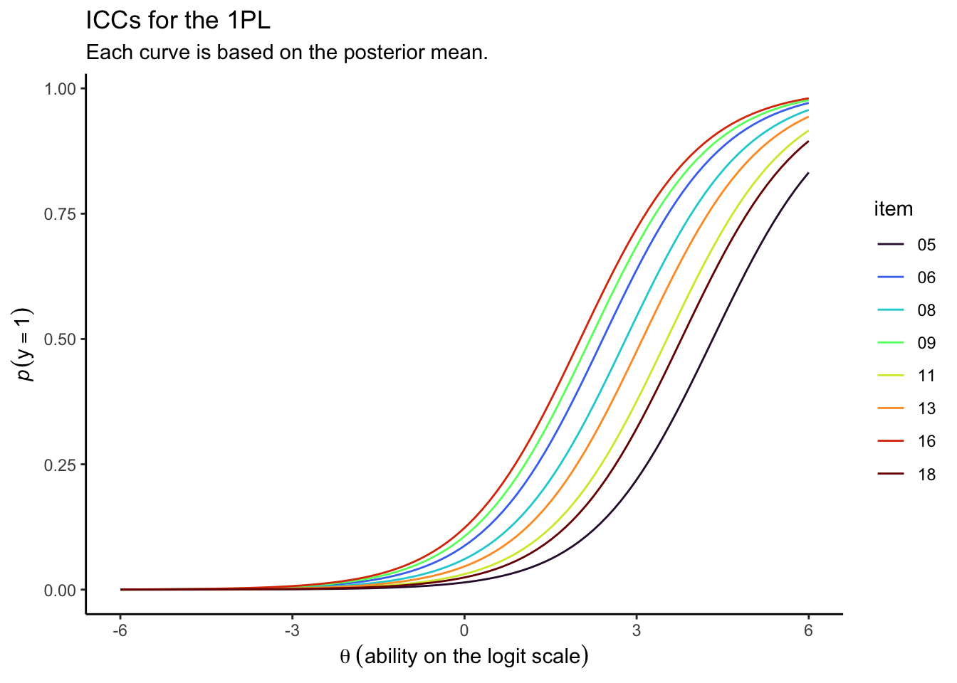
Since each item had a relatively low response probability, you have to go pretty far into the right-hand side of the \(\theta\) range before the curves start to approach the top of the \(y\) axis.
To make the ICCs for the 2PL model, the data wrangling will require a couple more steps. First, we extract the posterior draws and take a quick look at the columns of interest.
draws <- as_draws_df(irt2)

# what do we care about?
draws %>%
  select(.draw, b_eta_Intercept, b_logalpha_Intercept, starts_with("r_item")) %>%
  glimpse()
## Rows: 4,000
## Columns: 19
## $ .draw                            <int> 1, 2, 3, 4, 5, 6, 7, 8, 9, 10, 11, 12, 13, 14, 15, 16, 17, 18, 19, …
## $ b_eta_Intercept                  <dbl> -1.3855075, -1.4968294, -1.6918246, -1.6252046, -1.7095222, -1.4090…
## $ b_logalpha_Intercept             <dbl> 0.7814705, 0.6435611, 0.3971659, 0.5084503, 0.7547493, 1.2154113, 1…
## $ `r_item__eta[05,Intercept]`      <dbl> -0.7922848, -0.7423704, -1.1893399, -1.0718978, -0.2636685, -0.3965…
## $ `r_item__eta[06,Intercept]`      <dbl> 0.26895443, 0.21153136, 0.24488884, 0.20332673, 0.52650711, 0.51766…
## $ `r_item__eta[08,Intercept]`      <dbl> 0.1730248531, -0.0251183662, 0.0966877581, -0.0626794892, 0.3235805…
## $ `r_item__eta[09,Intercept]`      <dbl> 0.50089389, 0.39236895, 0.35678623, 0.41680088, 0.66285740, 0.53730…
## $ `r_item__eta[11,Intercept]`      <dbl> -0.17619531, -1.00068058, -0.41426442, -0.71686852, -0.15409689, -0…
## $ `r_item__eta[13,Intercept]`      <dbl> 0.02890276, -0.19689487, 0.12965889, -0.13639774, 0.35999998, 0.250…
## $ `r_item__eta[16,Intercept]`      <dbl> 0.5650797, 0.3484697, 0.5692639, 0.4691862, 0.5286982, 0.7387770, 0…
## $ `r_item__eta[18,Intercept]`      <dbl> -0.03100911, -0.94785287, -0.40602161, -1.06680784, -0.29232278, 0.…
## $ `r_item__logalpha[05,Intercept]` <dbl> -0.445733584, -0.168897075, -0.175487957, -0.023652177, -0.38447241…
## $ `r_item__logalpha[06,Intercept]` <dbl> 0.106865933, 0.183709540, 0.352641061, 0.372592174, 0.606879092, 0.…
## $ `r_item__logalpha[08,Intercept]` <dbl> 0.279715442, 0.224570579, 0.613387942, 0.344415036, 0.249641920, -0…
## $ `r_item__logalpha[09,Intercept]` <dbl> 0.46984590, 0.59974910, 0.61973239, 0.57372330, 0.67782554, 0.38758…
## $ `r_item__logalpha[11,Intercept]` <dbl> -0.23306444, -0.85055396, -0.31303715, -0.60098567, -0.40559846, -0…
## $ `r_item__logalpha[13,Intercept]` <dbl> -0.008225223, 0.116253481, 0.122579334, 0.291166675, 0.689798894, 0…
## $ `r_item__logalpha[16,Intercept]` <dbl> 0.092113896, 0.104240677, 0.092359783, 0.097844755, 0.494488271, 0.…
## $ `r_item__logalpha[18,Intercept]` <dbl> 0.09498269, -0.15278053, 0.01792382, -0.01208098, -0.31325790, -0.0…
Now there are 16 r_item__ columns, half of which correspond to the \(\xi_i\) deviations and the other half of which correspond to the \(\alpha_i\) deviations. In addition, we also have the b_logalpha_Intercept columns to contend with. So this time, we’ll follow up our pivot_longer() code with subsequent mutate() and select() steps, and complete the task with pivot_wider().
draws <- draws %>%
  select(.draw, b_eta_Intercept, b_logalpha_Intercept, starts_with("r_item")) %>%
  pivot_longer(starts_with("r_item")) %>%
  mutate(item      = str_extract(name, "\\d+"),
         parameter = ifelse(str_detect(name, "eta"), "xi", "logalpha")) %>%
  select(-name) %>%
  pivot_wider(names_from = parameter, values_from = value)

# what does this look like, now?
head(draws)
## # A tibble: 6 × 6
##   .draw b_eta_Intercept b_logalpha_Intercept item       xi logalpha
##   <int>           <dbl>                <dbl> <chr>   <dbl>    <dbl>
## 1     1           -1.39                0.781 05    -0.792  -0.446
## 2     1           -1.39                0.781 06     0.269   0.107
## 3     1           -1.39                0.781 08     0.173   0.280
## 4     1           -1.39                0.781 09     0.501   0.470
## 5     1           -1.39                0.781 11    -0.176  -0.233
## 6     1           -1.39                0.781 13     0.0289 -0.00823
With this configuration, it’s only a little more complicated to compute the probability summaries.
draws <- draws %>%
  expand(nesting(.draw, b_eta_Intercept, b_logalpha_Intercept, item, xi, logalpha),
         theta = seq(from = -6, to = 6, length.out = 100)) %>%
  # note the difference in the equation
  mutate(p = inv_logit_scaled(exp(b_logalpha_Intercept + logalpha) * (b_eta_Intercept + theta + xi))) %>%
  group_by(theta, item) %>%
  summarise(p = mean(p))

# what have we done?
head(draws)
## # A tibble: 6 × 3
## # Groups:   theta [1]
##   theta item           p
##   <dbl> <chr>      <dbl>
## 1    -6 05    0.0000152
## 2    -6 06    0.00000543
## 3    -6 08    0.00000967
## 4    -6 09    0.00000105
## 5    -6 11    0.000127
## 6    -6 13    0.00000111
And we plot.
draws %>%
  ggplot(aes(x = theta, y = p, color = item)) +
  geom_line() +
  scale_color_viridis_d(option = "H") +
  labs(title = "ICCs for the 2PL",
       subtitle = "Each curve is based on the posterior mean.",
       x = expression(theta~('ability on the logit scale')),
       y = expression(italic(p)(y==1))) +
  theme_classic()
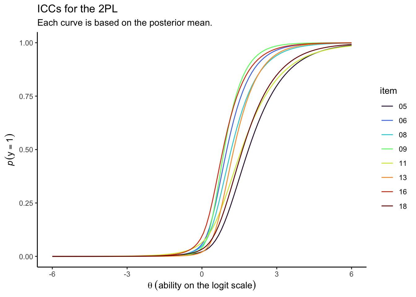
Looks like those \(\alpha_i\) parameters made a big difference for the ICCs.
IICs.
From a computational standpoint, item information curves (IICs) are a transformation of the ICCs. Recall that the \(y\) axis for the ICC is \(p\), the probability \(y = 1\) for a given item. For the IIC plots, the \(y\) axis shows information, which is a simple transformation of \(p\), following the form
$$\text{information} = p(1 - p).$$
So here’s how to use that equation and make the IIC plot for our 1PL model.
# these wrangling steps are all the same as before
as_draws_df(irt1) %>%
  select(.draw, b_Intercept, starts_with("r_item")) %>%
  pivot_longer(starts_with("r_item"), names_to = "item", values_to = "xi") %>%
  mutate(item = str_extract(item, "\\d+")) %>%
  expand(nesting(.draw, b_Intercept, item, xi),
         theta = seq(from = -6, to = 6, length.out = 200)) %>%
  mutate(p = inv_logit_scaled(b_Intercept + xi + theta)) %>%

  # this part, right here, is what's new
  mutate(i = p * (1 - p)) %>%
  group_by(theta, item) %>%
  summarise(i = median(i)) %>%

  # now plot!
  ggplot(aes(x = theta, y = i, color = item)) +
  geom_line() +
  scale_color_viridis_d(option = "H") +
  labs(title = "IICs for the 1PL",
       subtitle = "Each curve is based on the posterior median.",
       x = expression(theta~('ability on the logit scale')),
       y = "information") +
  theme_classic()
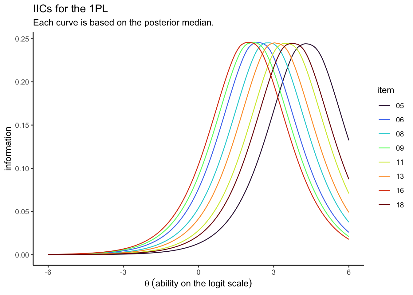
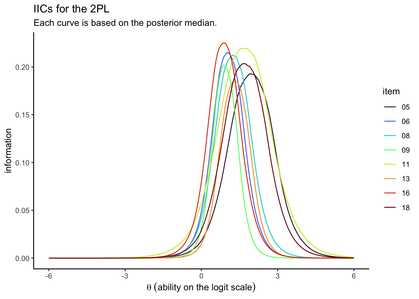
For kicks and giggles, we used the posterior medians, rather than the means. It’s similarly easy to compute the item-level information for the 2PL.
# these wrangling steps are all the same as before
as_draws_df(irt2) %>%
  select(.draw, b_eta_Intercept, b_logalpha_Intercept, starts_with("r_item")) %>%
  pivot_longer(starts_with("r_item")) %>%
  mutate(item      = str_extract(name, "\\d+"),
         parameter = ifelse(str_detect(name, "eta"), "xi", "logalpha")) %>%
  select(-name) %>%
  pivot_wider(names_from = parameter, values_from = value) %>%
  expand(nesting(.draw, b_eta_Intercept, b_logalpha_Intercept, item, xi, logalpha),
         theta = seq(from = -6, to = 6, length.out = 200)) %>%
  mutate(p = inv_logit_scaled(exp(b_logalpha_Intercept + logalpha) * (b_eta_Intercept + theta + xi))) %>%

  # again, here's the new part
  mutate(i = p * (1 - p)) %>%
  group_by(theta, item) %>%
  summarise(i = median(i)) %>%

  # now plot!
  ggplot(aes(x = theta, y = i, color = item)) +
  geom_line() +
  scale_color_viridis_d(option = "H") +
  labs(title = "IICs for the 2PL",
       subtitle = "Each curve is based on the posterior median.",
       x = expression(theta~('ability on the logit scale')),
       y = "information") +
  theme_classic()
TIC.
Sometimes researchers want to get a overall sense of the information in a group of items. For simplicity, here, we’ll just call groups of items a test. The test information curve (TIC) is a special case of the IIC, but applied to the whole test. In short, you compute the TIC by summing up the information for the individual items at each level of \(\theta\). Using the 1PL as an example, here’s how we might do that by hand.
as_draws_df(irt1) %>%
  select(.draw, b_Intercept, starts_with("r_item")) %>%
  pivot_longer(starts_with("r_item"), names_to = "item", values_to = "xi") %>%
  mutate(item = str_extract(item, "\\d+")) %>%
  expand(nesting(.draw, b_Intercept, item, xi),
         theta = seq(from = -6, to = 6, length.out = 200)) %>%
  mutate(p = inv_logit_scaled(b_Intercept + xi + theta)) %>%
  mutate(i = p * (1 - p)) %>%

  # this is where the TIC magic happens
  group_by(theta, .draw) %>%
  summarise(sum_i = sum(i)) %>%
  group_by(theta) %>%
  summarise(i = median(sum_i)) %>%

  # we plot
  ggplot(aes(x = theta, y = i)) +
  geom_line() +
  labs(title = "The test information curve for the 1PL",
       subtitle = "The curve is based on the posterior median.",
       x = expression(theta~('ability on the logit scale')),
       y = "information") +
  theme_classic()
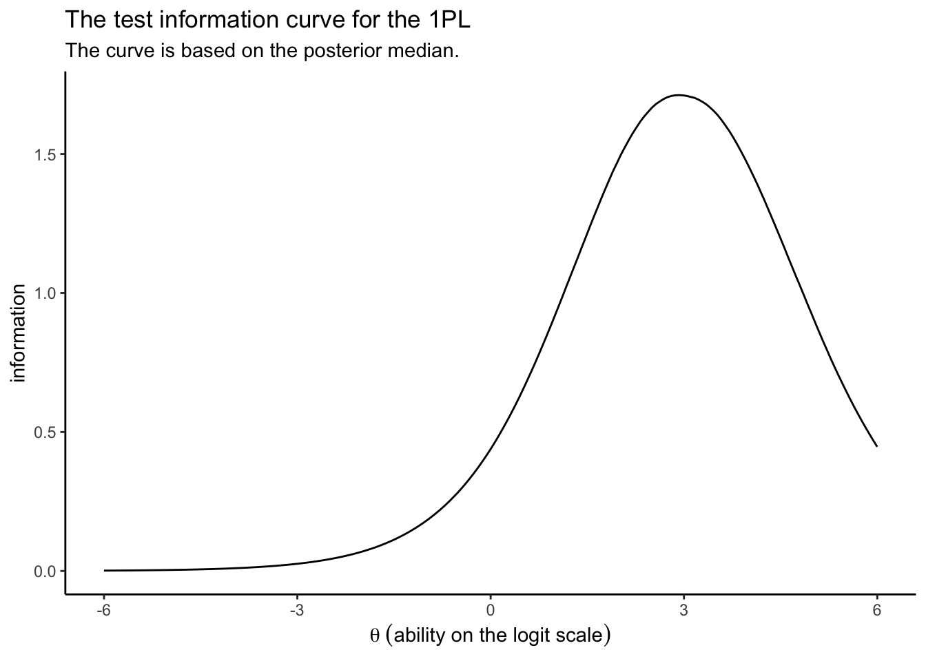
Taken as a whole, the combination of the eight items Loram et al. (
2019) settled on does a reasonable job differentiating among those with high \(\theta_p\) values. But this combination of items isn’t going to be the best at differentiating among those on the lower end of the \(\theta\) scale. You might say these eight items make for a difficult test.
Our method of extending the 1PL IIC to the TIC should work the same for the 2PL. I’ll leave it as an exercise for the interested reader.
Overview
We might outlines the steps in this post as:
- Fit your brms IRT model.
- Inspect the model with all your standard quality checks (e.g.,
\(\widehat R\)values, trace plots). - Extract your posterior draws with the
as_draws_df()function. - Isolate the item-related columns. Within the multilevel IRT context, this will typically involve an overall intercept (e.g.,
b_Interceptfor our 1PLirt1) and item-specific deviations (e.g., the columns starting withr_itemin our 1PLirt1). - Arrange the data into a format that makes it easy to add the overall intercept in question to each of the item-level deviations in question. For me, this seemed easiest with the long format via the
pivot_longer()function. - Expand the data over a range of ability
\((\theta)\)values. For me, this worked well with theexpand()function. - Use the model-implied formula to compute the
\(p(y = 1)\). - Group the results by item and
\(\theta\)and summarize the\(p(y = 1)\)distributions with something like the mean or median. - Plot the results with
ggplot2::geom_line()and friends.
Next steps
You should be able to generalize this workflow to IRT models for data with more than two categories. You’ll just have to be careful about juggling your thresholds. You might find some inspiration along these lines here and here.
You could totally switch up this workflow to use some of the data wrangling helpers from the tidybayes package ( Kay, 2022). That could be a nifty little blog post in and of itself.
One thing that’s super lame about conventional ICC/IIC plots is there’s no expression of uncertainty. To overcome that, you could compute the 95% intervals (or 50% or whatever) in the same summarise() line where you computed the mean and then express those interval bounds with something like geom_ribbon() in your plot. The difficulty I foresee is it will result in overplotting for any models with more than like five items. Perhaps faceting would be the solution, there.
I’m no IRT jock and may have goofed some of the steps or equations. To report mistakes or provide any other constructive criticism, just chime in on this Twitter thread:
New blog up!https://t.co/ZOy9Cxrqat
— Solomon Kurz (@SolomonKurz) June 29, 2021
This time we practice making ICC plots for #brms-based multilevel IRT models.
Session info
sessionInfo()
## R version 4.2.0 (2022-04-22)
## Platform: x86_64-apple-darwin17.0 (64-bit)
## Running under: macOS Big Sur/Monterey 10.16
##
## Matrix products: default
## BLAS:   /Library/Frameworks/R.framework/Versions/4.2/Resources/lib/libRblas.0.dylib
## LAPACK: /Library/Frameworks/R.framework/Versions/4.2/Resources/lib/libRlapack.dylib
##
## locale:
## [1] en_US.UTF-8/en_US.UTF-8/en_US.UTF-8/C/en_US.UTF-8/en_US.UTF-8
##
## attached base packages:
## [1] stats     graphics  grDevices utils     datasets  methods   base
##
## other attached packages:
##  [1] brms_2.18.0     Rcpp_1.0.9      forcats_0.5.1   stringr_1.4.1   dplyr_1.0.10    purrr_0.3.4
##  [7] readr_2.1.2     tidyr_1.2.1     tibble_3.1.8    ggplot2_3.4.0   tidyverse_1.3.2
##
## loaded via a namespace (and not attached):
##   [1] readxl_1.4.1         backports_1.4.1      plyr_1.8.7           igraph_1.3.4         splines_4.2.0
##   [6] crosstalk_1.2.0      TH.data_1.1-1        rstantools_2.2.0     inline_0.3.19        digest_0.6.30
##  [11] htmltools_0.5.3      fansi_1.0.3          magrittr_2.0.3       checkmate_2.1.0      googlesheets4_1.0.1
##  [16] tzdb_0.3.0           modelr_0.1.8         RcppParallel_5.1.5   matrixStats_0.62.0   xts_0.12.1
##  [21] sandwich_3.0-2       prettyunits_1.1.1    colorspace_2.0-3     rvest_1.0.2          haven_2.5.1
##  [26] xfun_0.35            callr_3.7.3          crayon_1.5.2         jsonlite_1.8.3       lme4_1.1-31
##  [31] survival_3.4-0       zoo_1.8-10           glue_1.6.2           gtable_0.3.1         gargle_1.2.0
##  [36] emmeans_1.8.0        distributional_0.3.1 pkgbuild_1.3.1       rstan_2.21.7         abind_1.4-5
##  [41] scales_1.2.1         mvtnorm_1.1-3        DBI_1.1.3            miniUI_0.1.1.1       viridisLite_0.4.1
##  [46] xtable_1.8-4         stats4_4.2.0         StanHeaders_2.21.0-7 DT_0.24              htmlwidgets_1.5.4
##  [51] httr_1.4.4           threejs_0.3.3        posterior_1.3.1      ellipsis_0.3.2       pkgconfig_2.0.3
##  [56] loo_2.5.1            farver_2.1.1         sass_0.4.2           dbplyr_2.2.1         utf8_1.2.2
##  [61] labeling_0.4.2       tidyselect_1.1.2     rlang_1.0.6          reshape2_1.4.4       later_1.3.0
##  [66] munsell_0.5.0        cellranger_1.1.0     tools_4.2.0          cachem_1.0.6         cli_3.4.1
##  [71] generics_0.1.3       broom_1.0.1          ggridges_0.5.3       evaluate_0.18        fastmap_1.1.0
##  [76] yaml_2.3.5           processx_3.8.0       knitr_1.40           fs_1.5.2             nlme_3.1-159
##  [81] mime_0.12            projpred_2.2.1       xml2_1.3.3           compiler_4.2.0       bayesplot_1.9.0
##  [86] shinythemes_1.2.0    rstudioapi_0.13      gamm4_0.2-6          reprex_2.0.2         bslib_0.4.0
##  [91] stringi_1.7.8        highr_0.9            ps_1.7.2             blogdown_1.15        Brobdingnag_1.2-8
##  [96] lattice_0.20-45      Matrix_1.4-1         nloptr_2.0.3         markdown_1.1         shinyjs_2.1.0
## [101] tensorA_0.36.2       vctrs_0.5.0          pillar_1.8.1         lifecycle_1.0.3      jquerylib_0.1.4
## [106] bridgesampling_1.1-2 estimability_1.4.1   httpuv_1.6.5         R6_2.5.1             bookdown_0.28
## [111] promises_1.2.0.1     gridExtra_2.3        codetools_0.2-18     boot_1.3-28          colourpicker_1.1.1
## [116] MASS_7.3-58.1        gtools_3.9.3         assertthat_0.2.1     withr_2.5.0          shinystan_2.6.0
## [121] multcomp_1.4-20      mgcv_1.8-40          parallel_4.2.0       hms_1.1.1            grid_4.2.0
## [126] coda_0.19-4          minqa_1.2.5          rmarkdown_2.16       googledrive_2.0.0    shiny_1.7.2
## [131] lubridate_1.8.0      base64enc_0.1-3      dygraphs_1.1.1.6
References
Albano, T. (2020). Introduction to educational and psychological measurement using R. https://www.thetaminusb.com/intro-measurement-r/
Bonifay, W. (2019). Multidimensional item response theory. SAGE Publications. https://us.sagepub.com/en-us/nam/multidimensional-item-response-theory/book257740
Bürkner, P.-C. (2020). Bayesian item response modeling in R with brms and Stan. http://arxiv.org/abs/1905.09501
Bürkner, P.-C. (2021). Estimating non-linear models with brms. https://CRAN.R-project.org/package=brms/vignettes/brms_nonlinear.html
Bürkner, P.-C. (2017). brms: An R package for Bayesian multilevel models using Stan. Journal of Statistical Software, 80(1), 1–28. https://doi.org/10.18637/jss.v080.i01
Bürkner, P.-C. (2018). Advanced Bayesian multilevel modeling with the R package brms. The R Journal, 10(1), 395–411. https://doi.org/10.32614/RJ-2018-017
Bürkner, P.-C. (2022). brms: Bayesian regression models using ’Stan’. https://CRAN.R-project.org/package=brms
Crocker, L., & Algina, J. (2006). Introduction to classical and modern test theory. Cengage Learning.
De Ayala, R. J. (2008). The theory and practice of item response theory. Guilford Publications. https://www.guilford.com/books/The-Theory-and-Practice-of-Item-Response-Theory/R-de-Ayala/9781593858698
Grolemund, G., & Wickham, H. (2017). R for data science. O’Reilly. https://r4ds.had.co.nz
Kay, M. (2022). tidybayes: Tidy data and ’geoms’ for Bayesian models. https://CRAN.R-project.org/package=tidybayes
Kruschke, J. K. (2015). Doing Bayesian data analysis: A tutorial with R, JAGS, and Stan. Academic Press. https://sites.google.com/site/doingbayesiandataanalysis/
Lewandowski, D., Kurowicka, D., & Joe, H. (2009). Generating random correlation matrices based on vines and extended onion method. Journal of Multivariate Analysis, 100(9), 1989–2001. https://doi.org/10.1016/j.jmva.2009.04.008
Loram, G., Ling, M., Head, A., & Clarke, E. J. R. (2019). Validation of a novel climate change denial measure using item response theory. https://doi.org/10.31234/osf.io/57nbk
McElreath, R. (2020). Statistical rethinking: A Bayesian course with examples in R and Stan (Second Edition). CRC Press. https://xcelab.net/rm/statistical-rethinking/
McElreath, R. (2015). Statistical rethinking: A Bayesian course with examples in R and Stan. CRC press. https://xcelab.net/rm/statistical-rethinking/
R Core Team. (2022). R: A language and environment for statistical computing. R Foundation for Statistical Computing. https://www.R-project.org/
Reckase, M. D. (2009). Multidimensional item response theory models. Springer. https://www.springer.com/gp/book/9780387899756
Wickham, H. (2022). tidyverse: Easily install and load the ’tidyverse’. https://CRAN.R-project.org/package=tidyverse
Wickham, H., Averick, M., Bryan, J., Chang, W., McGowan, L. D., François, R., Grolemund, G., Hayes, A., Henry, L., Hester, J., Kuhn, M., Pedersen, T. L., Miller, E., Bache, S. M., Müller, K., Ooms, J., Robinson, D., Seidel, D. P., Spinu, V., … Yutani, H. (2019). Welcome to the tidyverse. Journal of Open Source Software, 4(43), 1686. https://doi.org/10.21105/joss.01686
-
I should disclose that although I have not read through Bonifay’s ( 2019) text, he offered to send me a copy around the time I uploaded this post. ↩︎
-
Adopting the three-term multilevel structure–$\beta_0 + \theta_p + \xi_i$, where the latter two terms are
\(\operatorname{Normal}(0, \sigma_x)\)–places this form of the 1PL model squarely within the generalized linear multilevel model (GLMM). McElreath ( 2015, Chapter 12) referred to this particular model type as a cross-classified model. Coming from another perspective, Kruschke ( 2015, Chapter 19 and 20) described this as a kind of multilevel analysis of variance (ANOVA). ↩︎ -
For a nice blog post on the LKJ, check out Stephen Martin’s Is the LKJ(1) prior uniform? “Yes”. ↩︎
- Posted on:
- June 29, 2021
- Length:
- 26 minute read, 5398 words