Don't forget your inits

tl;dr

When your MCMC chains look a mess, you might have to manually set your initial values. If you’re a fancy pants, you can use a custom function.

Context

A collaborator asked me to help model some reaction-time data. One of the first steps was to decide on a reasonable likelihood function. You can see a productive Twitter thread on that process here. Although I’ve settled on the shifted-lognormal function, I also considered the exponentially modified Gaussian function (a.k.a. exGaussian). As it turns out, the exGaussian can be fussy to work with! After several frustrating attempts, I solved the problem by fiddling with my initial values. The purpose of this post is to highlight the issue and give you some options.

I make assumptions.

• This post is for Bayesians. For thorough introductions to contemporary Bayesian regression, I recommend either edition of McElreath’s text ( 2020, 2015); Kruschke’s ( 2015) text; or Gelman, Hill, and Vehtari’s ( 2020) text.
• Though not necessary, it will help if you’re familiar with multilevel regression. The texts by McElreath and Kruschke, from above, can both help with that.
• All code is in R ( R Core Team, 2022), with an emphasis on the brms package ( Bürkner, 2017, 2018, 2022). We will also make good use of the tidyverse ( Wickham et al., 2019; Wickham, 2022), the patchwork package ( Pedersen, 2022), and ggmcmc ( Fernández i Marín, 2016, 2021). We will also use the lisa package ( Littlefield, 2020) to select the color palette for our figures.

Load the primary R packages and adjust the global plotting theme defaults.

# load
library(tidyverse)
library(brms)
library(patchwork)
library(ggmcmc)
library(lisa)

# define the color palette
fk <- lisa_palette("FridaKahlo", n = 31, type = "continuous")

# adjust the global plotting theme
theme_set(
  theme_gray(base_size = 13) +
    theme(
      text = element_text(family = "Times", color = fk[1]),
      axis.text = element_text(family = "Times", color = fk[1]),
      axis.ticks = element_line(color = fk[1]),
      legend.background = element_blank(),
      legend.box.background = element_blank(),
      legend.key = element_blank(),
      panel.background = element_rect(fill = alpha(fk[16], 1/4), color = "transparent"),
      panel.grid = element_blank(),
      plot.background = element_rect(fill = alpha(fk[16], 1/4), color = "transparent")
    )
)

The color palette in this post is inspired by Frida Kahlo’s Self-Portrait with Thorn Necklace and Hummingbird.

We need data

I’m not at liberty to share the original data. However, I have simulated a new data set that has the essential features of the original and I have saved the file on GitHub. You can load it like this.

load(url("https://github.com/ASKurz/blogdown/raw/main/content/blog/2021-06-05-don-t-forget-your-inits/data/dat.rda?raw=true"))

# what is this?
glimpse(dat)

## Rows: 29,281
## Columns: 2
## $ id <chr> "a", "a", "a", "a", "a", "a", "a", "a", "a", "a", "a", "a", "a", "a", "a", "a", "a", "a", "a", "a…
## $ rt <dbl> 689.0489, 552.8998, 901.0891, 992.2104, 1218.2256, 1356.5888, 679.0385, 663.7340, 771.3938, 996.2…

Our primary variable of interest is rt, which is simulated reaction times in milliseconds. The reaction times are nested within 26 participants, who are denoted by the id column. The data are not balanced.

dat %>% 
  count(id, name = "trials") %>% 
  count(trials)

## # A tibble: 7 × 2
##   trials     n
##    <int> <int>
## 1    320     2
## 2    640     4
## 3    960     3
## 4   1121     1
## 5   1280    14
## 6   1600     1
## 7   2560     1

Whereas most participants have 1,280 trials, their numbers range from 320 to 2,560, which means we’ll want a multilevel model.

We can describe the data with the exGaussian function

To start getting a sense of the rt data, we’ll make a density plot of the overall distribution.

dat %>% 
  ggplot(aes(x = rt)) +
  geom_density(fill = fk[3], color = fk[3])

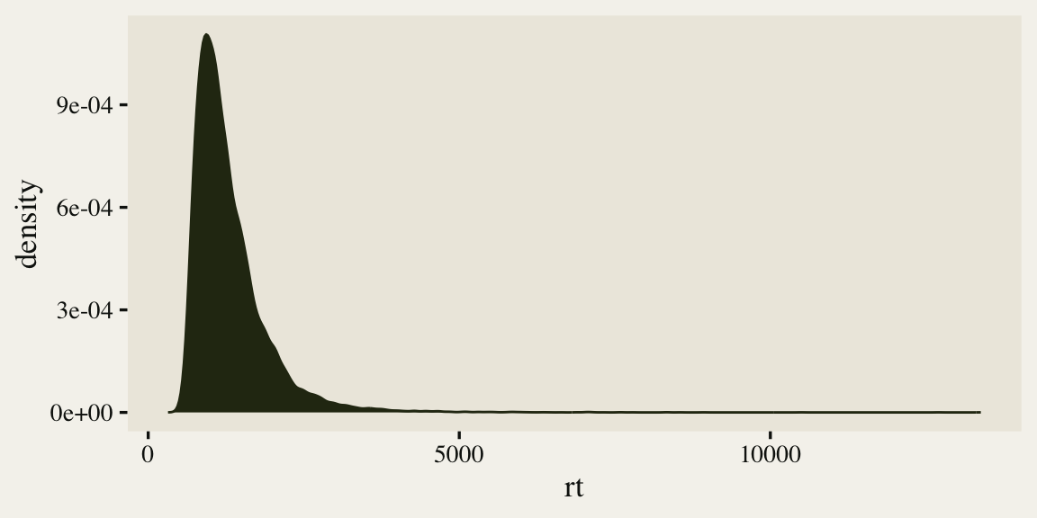
As is typical of reaction times, the data are continuous, non-negative, and strongly skewed to the right. There are any number of likelihood functions one can use to model data of this kind. One popular choice is the exGaussian. The exGaussian distribution has three parameters: \(\mu\), \(\sigma\), and \(\beta\)¹. The \(\mu\) and \(\sigma\) parameters govern the mean and standard deviation for the central Gaussian portion of the distribution. The \(\beta\) parameter governs the rate of the exponential distribution, which is tacked on to the right-hand side of the distribution. Within R, you can compute the density of various exGaussian distributions using the brms::dexgaussian() function. If you fool around with the parameter settings, a bit, you can make an exGaussian curve that fits pretty closely to the shape of our rt data. For example, here’s what it looks like when we set mu = 1300, sigma = 150, and beta = 520.

tibble(rt = seq(from = 0, to = 5500, length.out = 300),
       d = dexgaussian(rt, mu = 1300, sigma = 150, beta = 520)) %>% 
  
  ggplot(aes(x = rt)) +
  geom_density(data = dat,
               fill = fk[3], color = fk[3]) +
  geom_line(aes(y = d), 
            color = fk[31], linewidth = 5/4) +
  # zoom in on the bulk of the values
  coord_cartesian(xlim = c(0, 5000))

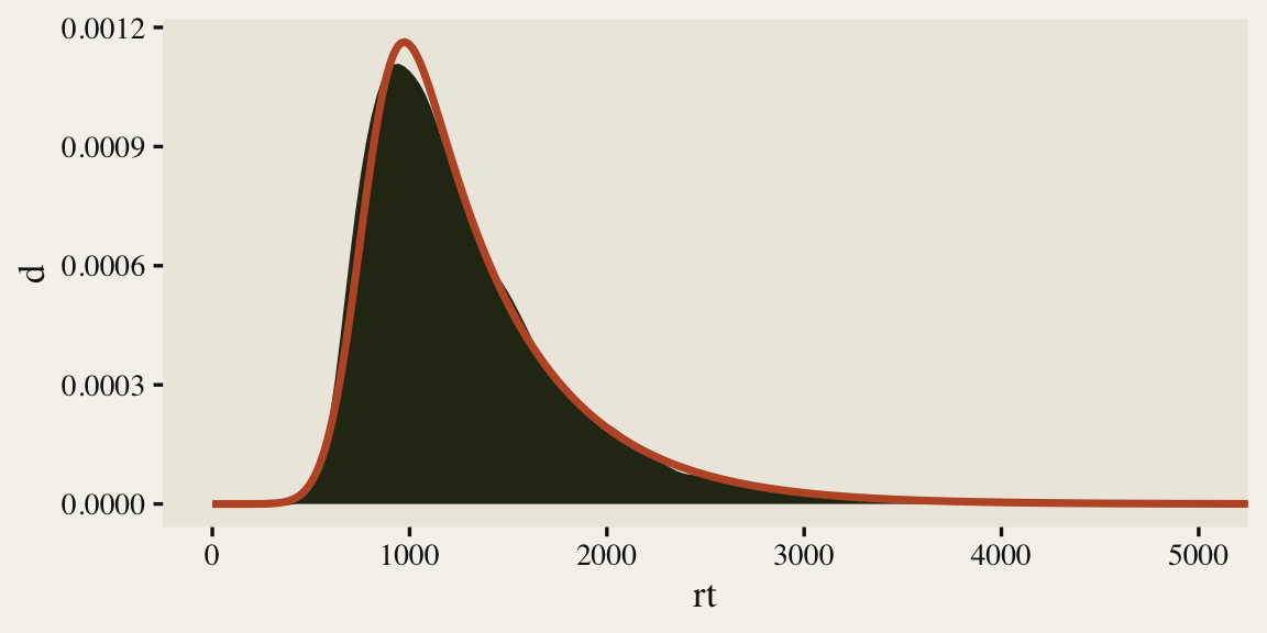
The fit isn’t perfect, but it gives a sense of where things are headed. It’s time to talk about modeling.

Models

In this post, we will explore three options for modeling the reaction-time data. The first will use default options. The second option will employ manually-set starting points. For the third option, we will use pseudorandom number generators to define the starting points, all within a custom function.

Model 1: Use the exGaussian with default settings.

When using brms, you can fit an exGaussian model by setting family = exgaussian(). Here we’ll allow the \(\mu\) parameters to vary by participant, but keep the \(\sigma\) and \(\beta\) parameters fixed.

fit1 <- brm(
  data = dat,
  family = exgaussian(),
  formula = rt ~ 1 + (1 | id),
  cores = 4, seed = 1
)

I’m not going to show them all, here, for the sake of space, but this model returned warnings about 604 transitions, 1 chain for which the estimated Bayesian Fraction of Missing Information was low, a large R-hat value of 2.85, and low bulk and tail effective sample sizes. In other words, this was a disaster. To help bring these all into focus, we’ll want to take a look at the chains in a trace plot. Since we’ll be doing this a few times, let’s go ahead and make a custom trace plot geom to suit our purposes. We’ll call it geom_trace().

geom_trace <- function(subtitle = NULL, 
                       xlab = "iteration", 
                       xbreaks = 0:4 * 500) {
  
  list(
    annotate(geom = "rect", 
             xmin = 0, xmax = 1000, ymin = -Inf, ymax = Inf,
             fill = fk[16], alpha = 1/2, linewidth = 0),
    geom_line(linewidth = 1/3),
    scale_color_manual(values = fk[c(3, 8, 27, 31)]),
    scale_x_continuous(xlab, breaks = xbreaks, expand = c(0, 0)),
    labs(subtitle = subtitle),
    theme(panel.grid = element_blank())
  )
  
}

For your real-world models, it’s good to look at the tract plots for all major model parameters. Here we’ll just focus on the \(\mu\) intercept.

p1 <- ggs(fit1, burnin = TRUE) %>%
  filter(Parameter == "b_Intercept") %>% 
  mutate(chain = factor(Chain),
         intercept = value) %>% 
  
  ggplot(aes(x = Iteration, y = intercept, color = chain)) +
  geom_trace(subtitle = "fit1 (default settings)") +
  scale_y_continuous(breaks = c(0, 650, 1300), limits = c(NA, 1430))

p1

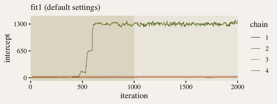
Since we pulled the chains using the ggmcmc::ggs() function, we were able to plot the warmup iterations (darker beige background on the left) along with the post-warmup iterations (lighter beige background on the right). Although one of our chains eventually made its way to the posterior, three out of the four stagnated near their starting values. This brings us to a major point in this post: Starting points can be a big deal.

Starting points can be a big deal.

I’m not going to go into the theory underlying Markov chain Monte Carlo (MCMC) methods in any detail. For that, check out some of the latter chapters in Gill ( 2015) or Gelman et al. ( 2013). In brief, if you run a Markov chain for an infinite number of iterations, it will converge on the correct posterior distribution. The problem is we can’t run our chains for that long, which means we have to be careful about whether our finite-length chains have converged properly. Starting points are one of the factors that can influence this process.

One of the ways to help make sure your MCMC chains are sampling well is to run multiple chains for a while and check to see whether they have all converged around the same parameter space. Ideally, each chain will start from a different initial value. In practice, the first several iterations following the starting values are typically discarded. With older methods, like the Gibbs sampler, this was called the “burn-in” period. With Hamiltonian Monte Carlo (HMC), which is what brms uses, we have a similar period called “warmup.” When everything goes well, the MCMC chains will all have traversed from their starting values to sampling probabilistically from the posterior distribution once they have emerged from the warmup phase. However, this isn’t always the case. Sometimes the chains get stuck around their stating values and continue to linger there, even after you have terminated the warmup period. When this happens, you’ll end up with samples that are still tainted by their starting values and are not yet representative of the posterior distribution.

In our example, above, we used the brms default settings of four chains, each of which ran for 1,000 warmup iterations and then 1,000 post-warmup iterations. We also used the brms default for the starting values. These defaults are based on the Stan defaults, which is to randomly select the starting points from a uniform distribution ranging from -2 to 2. For details, see the Random initial values section of the Stan Reference Manual ( Stan Development Team, 2021).

In my experience, the brms defaults are usually pretty good. My models often quickly traverse from their starting values to concentrate in the posterior, just like our second chain did, above. When things go wrong, sometimes adding stronger priors can work. Other times it makes sense to rescale or reparameterize the model, somehow. In this case, I have reasons to want to (a) use default priors and to (b) stick to the default parameterization applied to the transformed data. Happily, we have another trick at out disposal: We can adjust the starting points.

Within brms::brm(), we can control the starting values with the inits argument. The default is inits = "random", which follows the Stan convention of sampling from \((-2, 2)\), as discussed above. Another option is to fix all starting values to zero by setting inits = "0". This often works surprisingly well, but it wasn’t the solution in this case. If you look at the trace plot, above, you’ll see that all the starting values are a long ways from the target range, which is somewhere around 1,300. So why not just put the starting values near there?

Model 2: Fit the model with initial values set by hand.

When you specify start values for the parameters in your Stan models, you need to do so with a list of lists. Each MCMC chain will need its own list. In our case, that means we’ll need four separate lists, each of which will be nested within a single higher-order list. For example, here we’ll define a single list called inits, which will have starting values defined for our primary three population-level parameters.

inits <- list(
  Intercept = 1300,
  sigma     = 150,
  beta      = 520
  )

# what is this?
inits

## $Intercept
## [1] 1300
## 
## $sigma
## [1] 150
## 
## $beta
## [1] 520

Notice that we didn’t bother setting a starting value for the standard-deviation parameter for the random intercepts. That parameter, then, will just get the brms default. The others will the the start values, as assigned. Now, since we have four chains to assign start values to, a quick and dirty method is to just use the same ones for all four chains. Here’s how to do that.

list_of_inits <- list(inits, inits, inits, inits)

Our list_of_inits object is a list into which we have saved four copies of our inits list. Here’s how to use those values within brms::brm(). Just plug them into the inits argument.

fit2 <- brm(
  data = dat,
  family = exgaussian(),
  formula = rt ~ 1 + (1 | id),
  cores = 4, seed = 1,
  inits = list_of_inits
)

The effective sample sizes are still a little low, but the major pathologies are now gone. Compare the updated traceplot for the intercept to the first one.

# adjust fit1
p1 <- p1 +
  geom_trace(subtitle = "fit1 (default settings)",
             xlab = NULL, xbreaks = NULL)

# fit2
p2 <- ggs(fit2) %>%
  filter(Parameter == "b_Intercept") %>% 
  mutate(chain = factor(Chain),
         intercept = value) %>% 
  
  ggplot(aes(x = Iteration, y = intercept, color = chain)) +
  geom_trace(subtitle = "fit2 (manual copy/paste inits settings)") +
  coord_cartesian(ylim = c(1200, 1400))

# combine
p1 / p2

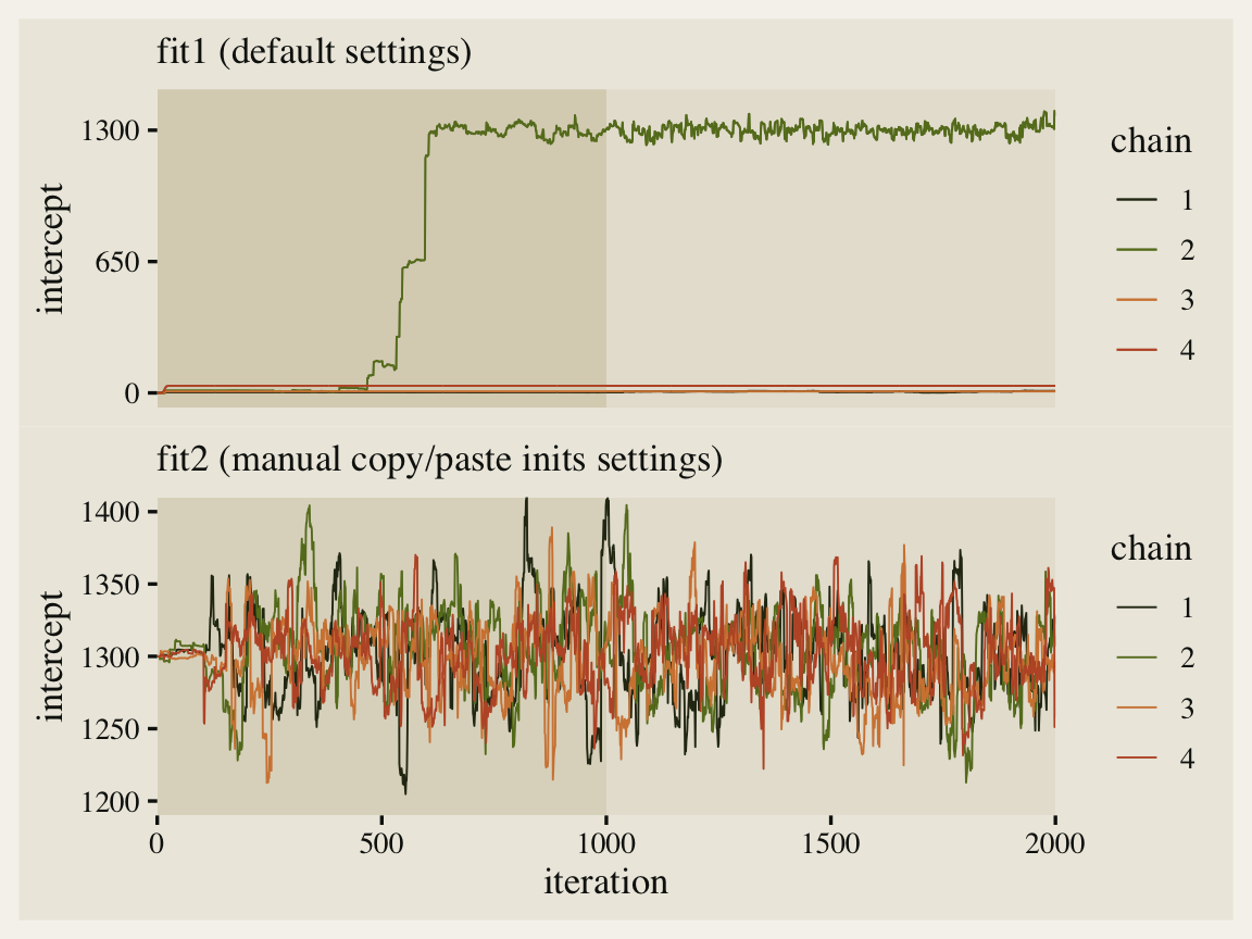
Man that looks better! See how all four of our chains started out at 1,300? That’s because of how we copy/pasted inits four times within our list_of_inits object. This is kinda okay, but we can do better.

Model 3: Set the initial values with a custom function.

Returning back to MCMC theory, a bit, it’s generally a better idea to assign each chain its own starting value. Then, if all chains converge into the same part in the parameter space, that provides more convincing evidence they’re all properly exploring the posterior. To be clear, this isn’t rigorous evidence. It’s just better evidence than if we started them all in the same spot.

One way to give each chain its own starting value would be to manually set them. Here’s what that would look like if we were only working with two chains.

# set the values for the first chain
inits1 <- list(
  Intercept = 1250,
  sigma     = 140,
  beta      = 500
  )

# set new values for the second chain
inits2 <- list(
  Intercept = 1350,
  sigma     = 160,
  beta      = 540
  )

# combine the two lists into a single list
list_of_inits <- list(inits1, inits2)

This approach will work fine, but it’s tedious, especially if you’d like to apply it to a large number of parameters. A more programmatic approach would be to use a pseudorandom number-generating function to randomly set the starting values. Since the intercept is an unbounded parameter, the posterior for which will often look Gaussian, the rnorm() function can be a great choice for selecting its starting values. Since both \(\sigma\) and \(\beta\) parameters need to be non-negative, a better choice might be the runif() or rgamma() functions. Here we’ll just use runif() for each.

Since we’re talking about using the pseudorandom number generators to pick our values, it would be nice if the results were reproducible. We can do that by working in the set.seed() function. Finally, it would be really sweet if we had a way to wrap set.seed() and the various number-generating functions into a single higher-order function. Here’s one way to make such a function, which I’m calling set_inits().

set_inits <- function(seed = 1) {
  
  set.seed(seed)
  list(
    Intercept = rnorm(n = 1, mean = 1300, sd = 100),
    sigma     = runif(n = 1, min = 100, max = 200),
    beta      = runif(n = 1, min = 450, max = 550)
  )
  
}

# try it out
set_inits(seed = 0)

## $Intercept
## [1] 1426.295
## 
## $sigma
## [1] 137.2124
## 
## $beta
## [1] 507.2853

Notice how we set the parameters within the rnorm() and runif() functions to values that seemed reasonable given our model. These values aren’t magic and you could adjust them to your own needs. Now, here’s how to use our handy set_inits() function to choose similar, but distinct, starting values for each of our four chains. We save the results in a higher-order list called my_second_list_of_inits.

my_second_list_of_inits <- list(
  # different seed values will return different results
  set_inits(seed = 1),
  set_inits(seed = 2),
  set_inits(seed = 3),
  set_inits(seed = 4)
)

# what have we done?
str(my_second_list_of_inits)

## List of 4
##  $ :List of 3
##   ..$ Intercept: num 1237
##   ..$ sigma    : num 157
##   ..$ beta     : num 541
##  $ :List of 3
##   ..$ Intercept: num 1210
##   ..$ sigma    : num 157
##   ..$ beta     : num 467
##  $ :List of 3
##   ..$ Intercept: num 1204
##   ..$ sigma    : num 138
##   ..$ beta     : num 483
##  $ :List of 3
##   ..$ Intercept: num 1322
##   ..$ sigma    : num 129
##   ..$ beta     : num 478

Now just plug my_second_list_of_inits into the inits argument and fit the model.

fit3 <- brm(
  data = dat,
  family = exgaussian(),
  formula = rt ~ 1 + (1 | id),
  cores = 4, seed = 1,
  inits = my_second_list_of_inits
)

As with fit2, our fit3 came out okay. Let’s inspect the intercept parameter with a final trace plot.

# adjust fit2
p2 <- p2 +
  geom_trace(subtitle = "fit2 (manual copy/paste inits settings)",
             xlab = NULL, xbreaks = NULL)

# fit3
p3 <- ggs(fit3) %>%
  filter(Parameter == "b_Intercept") %>% 
  mutate(chain = factor(Chain),
         intercept = value) %>% 
  
  ggplot(aes(x = Iteration, y = intercept, color = chain)) +
  geom_trace(subtitle = "fit3 (inits by a custom function)") +
  coord_cartesian(ylim = c(1200, 1400))

# combine
p1 / p2 / p3

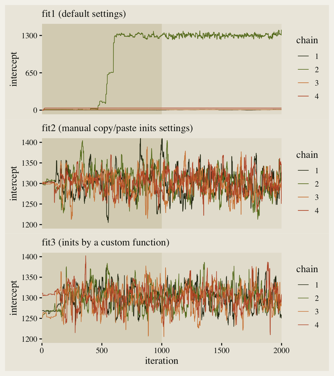
Now we have visual evidence that even though all four chains started at different places in the parameter space, they all converged into the same area. This still isn’t fully rigorous evidence our chains are performing properly, but it’s a major improvement from fit1 and a minor improvement from fit2. They aren’t shown here, but the same point holds for the \(\sigma\) and \(\beta\) parameters.

Okay, just for kicks and giggles, let’s see how well our last model did by way of a posterior predictive check.

bayesplot::color_scheme_set(fk[c(31, 31, 31, 3, 3, 3)])

pp_check(fit3, ndraws = 100) + 
  # we don't need to see the whole right tail
  coord_cartesian(xlim = c(0, 5000))

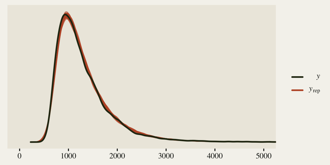
The model could be better, but it’s moving in the right direction and there don’t appear to be any major pathologies, like what we saw with fit1.

Recap

• If your try to fit a model with MCMC, you may sometimes end up with pathologies, such as divergent transitions, large numbers of transitions, high R-hat values, and/or very low effective sample size estimates.
• Sometimes these pathologies arise when the starting values for your chains are far away from the centers of their posterior densities.
• When using brms, you can solve this problem by setting the starting values with the inits argument.
• One approach is to manually set the starting values, saving them in a list of lists.
• Another approach is to use the pseudorandom number generators, such as rnorm() and runif(), to assign starting values within user-defined ranges.

Session info

sessionInfo()

## R version 4.2.0 (2022-04-22)
## Platform: x86_64-apple-darwin17.0 (64-bit)
## Running under: macOS Big Sur/Monterey 10.16
## 
## Matrix products: default
## BLAS:   /Library/Frameworks/R.framework/Versions/4.2/Resources/lib/libRblas.0.dylib
## LAPACK: /Library/Frameworks/R.framework/Versions/4.2/Resources/lib/libRlapack.dylib
## 
## locale:
## [1] en_US.UTF-8/en_US.UTF-8/en_US.UTF-8/C/en_US.UTF-8/en_US.UTF-8
## 
## attached base packages:
## [1] stats     graphics  grDevices utils     datasets  methods   base     
## 
## other attached packages:
##  [1] lisa_0.1.2      ggmcmc_1.5.1.1  patchwork_1.1.2 brms_2.18.0     Rcpp_1.0.9      forcats_0.5.1  
##  [7] stringr_1.4.1   dplyr_1.0.10    purrr_0.3.4     readr_2.1.2     tidyr_1.2.1     tibble_3.1.8   
## [13] ggplot2_3.4.0   tidyverse_1.3.2
## 
## loaded via a namespace (and not attached):
##   [1] readxl_1.4.1         backports_1.4.1      plyr_1.8.7           igraph_1.3.4         splines_4.2.0       
##   [6] crosstalk_1.2.0      TH.data_1.1-1        rstantools_2.2.0     inline_0.3.19        digest_0.6.30       
##  [11] htmltools_0.5.3      fansi_1.0.3          magrittr_2.0.3       checkmate_2.1.0      googlesheets4_1.0.1 
##  [16] tzdb_0.3.0           modelr_0.1.8         RcppParallel_5.1.5   matrixStats_0.62.0   xts_0.12.1          
##  [21] sandwich_3.0-2       prettyunits_1.1.1    colorspace_2.0-3     rvest_1.0.2          haven_2.5.1         
##  [26] xfun_0.35            callr_3.7.3          crayon_1.5.2         jsonlite_1.8.3       lme4_1.1-31         
##  [31] survival_3.4-0       zoo_1.8-10           glue_1.6.2           gtable_0.3.1         gargle_1.2.0        
##  [36] emmeans_1.8.0        distributional_0.3.1 pkgbuild_1.3.1       rstan_2.21.7         abind_1.4-5         
##  [41] scales_1.2.1         mvtnorm_1.1-3        GGally_2.1.2         DBI_1.1.3            miniUI_0.1.1.1      
##  [46] xtable_1.8-4         stats4_4.2.0         StanHeaders_2.21.0-7 DT_0.24              htmlwidgets_1.5.4   
##  [51] httr_1.4.4           threejs_0.3.3        RColorBrewer_1.1-3   posterior_1.3.1      ellipsis_0.3.2      
##  [56] reshape_0.8.9        pkgconfig_2.0.3      loo_2.5.1            farver_2.1.1         sass_0.4.2          
##  [61] dbplyr_2.2.1         utf8_1.2.2           labeling_0.4.2       tidyselect_1.1.2     rlang_1.0.6         
##  [66] reshape2_1.4.4       later_1.3.0          munsell_0.5.0        cellranger_1.1.0     tools_4.2.0         
##  [71] cachem_1.0.6         cli_3.4.1            generics_0.1.3       broom_1.0.1          ggridges_0.5.3      
##  [76] evaluate_0.18        fastmap_1.1.0        yaml_2.3.5           processx_3.8.0       knitr_1.40          
##  [81] fs_1.5.2             nlme_3.1-159         mime_0.12            projpred_2.2.1       xml2_1.3.3          
##  [86] compiler_4.2.0       bayesplot_1.9.0      shinythemes_1.2.0    rstudioapi_0.13      gamm4_0.2-6         
##  [91] reprex_2.0.2         bslib_0.4.0          stringi_1.7.8        highr_0.9            ps_1.7.2            
##  [96] blogdown_1.15        Brobdingnag_1.2-8    lattice_0.20-45      Matrix_1.4-1         nloptr_2.0.3        
## [101] markdown_1.1         shinyjs_2.1.0        tensorA_0.36.2       vctrs_0.5.0          pillar_1.8.1        
## [106] lifecycle_1.0.3      jquerylib_0.1.4      bridgesampling_1.1-2 estimability_1.4.1   httpuv_1.6.5        
## [111] R6_2.5.1             bookdown_0.28        promises_1.2.0.1     gridExtra_2.3        codetools_0.2-18    
## [116] boot_1.3-28          colourpicker_1.1.1   MASS_7.3-58.1        gtools_3.9.3         assertthat_0.2.1    
## [121] withr_2.5.0          shinystan_2.6.0      multcomp_1.4-20      mgcv_1.8-40          parallel_4.2.0      
## [126] hms_1.1.1            grid_4.2.0           coda_0.19-4          minqa_1.2.5          rmarkdown_2.16      
## [131] googledrive_2.0.0    shiny_1.7.2          lubridate_1.8.0      base64enc_0.1-3      dygraphs_1.1.1.6

References

Bürkner, P.-C. (2021). Parameterization of response distributions in brms. https://CRAN.R-project.org/package=brms/vignettes/brms_families.html
Bürkner, P.-C. (2017). brms: An R package for Bayesian multilevel models using Stan. Journal of Statistical Software, 80(1), 1–28. https://doi.org/10.18637/jss.v080.i01
Bürkner, P.-C. (2018). Advanced Bayesian multilevel modeling with the R package brms. The R Journal, 10(1), 395–411. https://doi.org/10.32614/RJ-2018-017
Bürkner, P.-C. (2022). brms: Bayesian regression models using ’Stan’. https://CRAN.R-project.org/package=brms
Fernández i Marín, X. (2016). ggmcmc: Analysis of MCMC samples and Bayesian inference. Journal of Statistical Software, 70(9), 1–20. https://doi.org/10.18637/jss.v070.i09
Fernández i Marín, X. (2021). ggmcmc: Tools for analyzing MCMC simulations from Bayesian inference [Manual]. https://CRAN.R-project.org/package=ggmcmc
Gelman, A., Carlin, J. B., Stern, H. S., Dunson, D. B., Vehtari, A., & Rubin, D. B. (2013). Bayesian data analysis (Third Edition). CRC press. https://stat.columbia.edu/~gelman/book/
Gelman, A., Hill, J., & Vehtari, A. (2020). Regression and other stories. Cambridge University Press. https://doi.org/10.1017/9781139161879
Gill, J. (2015). Bayesian methods: A social and behavioral sciences approach (Third Edition). CRC press. https://www.routledge.com/Bayesian-Methods-A-Social-and-Behavioral-Sciences-Approach-Third-Edition/Gill/p/book/9781439862483
Kruschke, J. K. (2015). Doing Bayesian data analysis: A tutorial with R, JAGS, and Stan. Academic Press. https://sites.google.com/site/doingbayesiandataanalysis/
Littlefield, T. (2020). lisa: Color palettes from color lisa [Manual]. https://CRAN.R-project.org/package=lisa
McElreath, R. (2020). Statistical rethinking: A Bayesian course with examples in R and Stan (Second Edition). CRC Press. https://xcelab.net/rm/statistical-rethinking/
McElreath, R. (2015). Statistical rethinking: A Bayesian course with examples in R and Stan. CRC press. https://xcelab.net/rm/statistical-rethinking/
Pedersen, T. L. (2022). patchwork: The composer of plots. https://CRAN.R-project.org/package=patchwork
R Core Team. (2022). R: A language and environment for statistical computing. R Foundation for Statistical Computing. https://www.R-project.org/
Stan Development Team. (2021). Stan reference manual, Version 2.27. https://mc-stan.org/docs/2_27/reference-manual/
Wickham, H. (2022). tidyverse: Easily install and load the ’tidyverse’. https://CRAN.R-project.org/package=tidyverse
Wickham, H., Averick, M., Bryan, J., Chang, W., McGowan, L. D., François, R., Grolemund, G., Hayes, A., Henry, L., Hester, J., Kuhn, M., Pedersen, T. L., Miller, E., Bache, S. M., Müller, K., Ooms, J., Robinson, D., Seidel, D. P., Spinu, V., … Yutani, H. (2019). Welcome to the tidyverse. Journal of Open Source Software, 4(43), 1686. https://doi.org/10.21105/joss.01686
-
There are different ways to parameterize the exGaussian distribution and these differences may involve different ways to express what we’re calling
\(\beta\). Since our parameterization is based on Paul Bürkner’s work, you might check out the Response time models section in his ( 2021) document, Parameterization of response distributions in brms. ↩︎
- Posted on:
- June 5, 2021
- Length:
- 18 minute read, 3775 words