Yes, you can fit an exploratory factor analysis with lavaan

Purpose

Just this past week, I learned that, Yes, you can fit an exploratory factor analysis (EFA) with lavaan ( Rosseel, 2012; Rosseel & Jorgensen, 2019). At the moment, this functionality is only unofficially supported, which is likely why many don’t know about it, yet. You can get the [un]official details at issue #112 on the lavaan GitHub repository ( https://github.com/yrosseel/lavaan). The purpose of this blog post is to make EFAs with lavaan even more accessible and web searchable by walking through a quick example.

Set up

First, load our focal package, lavaan, along with the tidyverse ( Wickham et al., 2019; Wickham, 2022).

library(tidyverse)
library(lavaan)

The data are a subset of the data from Arruda et al. ( 2020). You can find various supporting materials for their paper on the OSF at https://osf.io/kx2ym/. We will load¹ a subset of the data saved in their Base R - EFICA (manuscript and book chapter).RData file (available at https://osf.io/p3fs6/) called ds.

load("data/ds.rda")

# what is this?
dim(ds)

## [1] 3284  540

Here we extract a subset of the columns, rename them, and save the reduced data frame as d.

d <-
  ds %>% 
  select(ife_1:ife_65) %>% 
  set_names(str_c("y", 1:65))

Participants were \(N = 3{,}284\) parents of children or adolescents, in Brazil. The columns in our d data are responses to 65 items from the parent version of an “assessment tool developed to comprehensively assess dysfunctional behaviors related to” executive functioning, called the Executive function inventory for children and adolescents (EFICA; p. 5). On each item, the parents rated their kids on a 3-point Likert-type scale ranging from 0 (never) to 2 (always/almost always). To give a better sense of the items:

The Parents’ version (EFICA-P) encompassed behaviors especially performed at home, such as “Leaves the light on, door open or wet towels on top of the bed, even after being told several times”, “Explodes or gets angry when he/she is contradicted” and/or “Interrupts others, doesn’t know how to wait for his/her turn to talk.” (p. 5)

We won’t be diving into the substance of the paper, here. For that, see Arruda et al. ( 2020). But for data validation purposes, the items should only take on integers 0 through 2. Turns out that the data did contain a few coding errors, which we will convert to missing data, here.

d <-
  d %>% 
  mutate_at(vars(y1:y65), ~ifelse(. %in% c(0:2), ., NA))

Here are the overall distributions, collapsing across items.

d %>% 
  pivot_longer(everything()) %>% 
  count(value) %>% 
  mutate(percent = (100 * n / sum(n)) %>% round(digits = 1))

## # A tibble: 4 × 3
##   value     n percent
##   <dbl> <int>   <dbl>
## 1     0 85480    40  
## 2     1 94490    44.3
## 3     2 32276    15.1
## 4    NA  1214     0.6

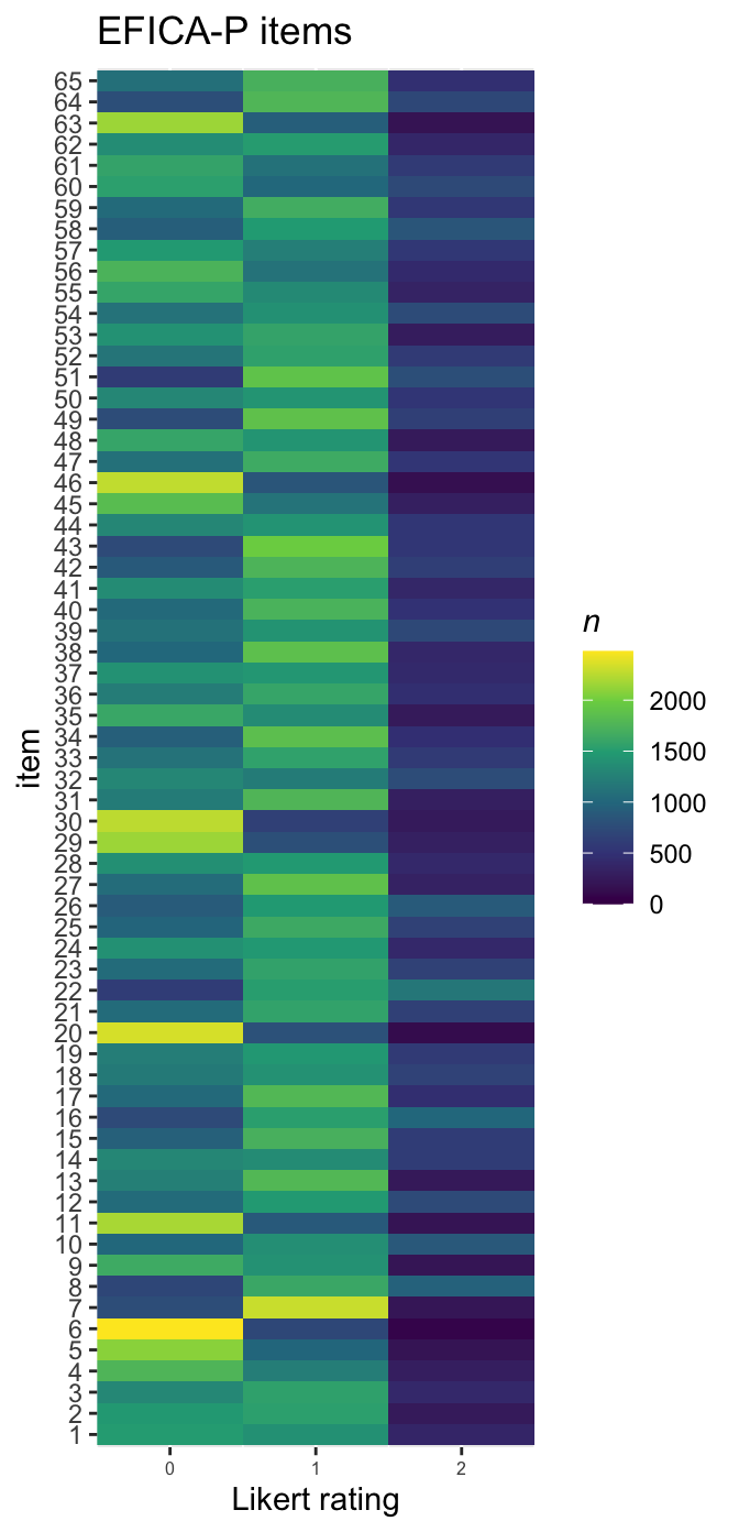
We might make a tile plot to get a sense high-level sense of the distributions across the items.

d %>% 
  pivot_longer(everything()) %>% 
  mutate(item = factor(name, 
                       levels = str_c("y", 1:65),
                       labels = 1:65)) %>% 
  count(item, value) %>% 
  
  ggplot(aes(x = value, y = item, fill = n)) +
  geom_tile() +
  scale_fill_viridis_c(expression(italic(n)), limits = c(0, NA)) +
  scale_x_continuous("Likert rating", expand = c(0, 0), breaks = 0:2) +
  ggtitle("EFICA-P items") +
  theme(axis.text.x = element_text(size = 6))

EFA in lavaan

Consider your estimation method.

An important preliminary step before fitting an EFA is getting a good sense of the data. In the last section, we learned the data are composed of three ordinal categories, which means that conventional estimators, such as maximum likelihood, won’t be the best of choices. Happily, lavaan offers several good options for ordinal data, which you can learn more about at https://lavaan.ugent.be/tutorial/cat.html and https://lavaan.ugent.be/tutorial/est.html. The default is the WLSMV estimator (i.e., estimator = "WLSMV"), which our friends in quantitative methodology have shown is generally a good choice (e.g., Flora & Curran, 2004; Li, 2016).

How many factors should we consider?

In the paper, Arruda and colleagues considered models with up to five factors. Here we’re going to keep things simple and consider between one and three. However, I’d be remiss not to mention that for real-world analyses, this step is important and possibly underappreciated. Decades of methodological work suggest that some of the widely-used heuristics for deciding on the number of factors (e.g., scree plots and the Kaiser criterion) aren’t as good as the lesser-used parallel analysis approach. For a gentle introduction to the topic, check out Schmitt ( 2011). Though we won’t make use of it, here, the psych package ( Revelle, 2022) offers some nice options for parallel analysis by way of the fa.parallel() function.

Finally, we fit a few EFAs.

It’s time to fit our three EFAs. When defining the EFA models within lavaan, the critical features are how one defines the factors on the left-hand side of the equations. Here we define the models for all 65 items.

# 1-factor model
f1 <- '
efa("efa")*f1 =~ y1 + y2 + y3 + y4 + y5 + y6 + y7 + y8 + y9 + y10 +
                   y11 + y12 + y13 + y14 + y15 + y16 + y17 + y18 + y19 + y20 + 
                   y21 + y22 + y23 + y24 + y25 + y26 + y27 + y28 + y29 + y30 +
                   y31 + y32 + y33 + y34 + y35 + y36 + y37 + y38 + y39 + y40 +
                   y41 + y42 + y43 + y44 + y45 + y46 + y47 + y48 + y49 + y50 +
                   y51 + y52 + y53 + y54 + y55 + y56 + y57 + y58 + y59 + y60 +
                   y61 + y62 + y63 + y64 + y65
'

# 2-factor model
f2 <- '
efa("efa")*f1 +
efa("efa")*f2 =~ y1 + y2 + y3 + y4 + y5 + y6 + y7 + y8 + y9 + y10 +
                   y11 + y12 + y13 + y14 + y15 + y16 + y17 + y18 + y19 + y20 + 
                   y21 + y22 + y23 + y24 + y25 + y26 + y27 + y28 + y29 + y30 +
                   y31 + y32 + y33 + y34 + y35 + y36 + y37 + y38 + y39 + y40 +
                   y41 + y42 + y43 + y44 + y45 + y46 + y47 + y48 + y49 + y50 +
                   y51 + y52 + y53 + y54 + y55 + y56 + y57 + y58 + y59 + y60 +
                   y61 + y62 + y63 + y64 + y65
'

# 3-factor model
f3 <- '
efa("efa")*f1 +
efa("efa")*f2 +
efa("efa")*f3 =~ y1 + y2 + y3 + y4 + y5 + y6 + y7 + y8 + y9 + y10 +
                   y11 + y12 + y13 + y14 + y15 + y16 + y17 + y18 + y19 + y20 + 
                   y21 + y22 + y23 + y24 + y25 + y26 + y27 + y28 + y29 + y30 +
                   y31 + y32 + y33 + y34 + y35 + y36 + y37 + y38 + y39 + y40 +
                   y41 + y42 + y43 + y44 + y45 + y46 + y47 + y48 + y49 + y50 +
                   y51 + y52 + y53 + y54 + y55 + y56 + y57 + y58 + y59 + y60 +
                   y61 + y62 + y63 + y64 + y65
'

Now we’ve defined the three EFA models, we can fit the actual EFAs. One can currently do so with either the cfa() or sem() functions. The default rotation method is oblique Geomin. If you’re not up on rotation methods, you might check out Sass & Schmitt ( 2010). Here we’ll give a nod to tradition and use oblique Oblimin by setting rotation = "oblimin". Also, note our use of ordered = TRUE, which explicitly tells lavaan::cfa() to treat all 65 of our items as ordinal.

efa_f1 <- 
  cfa(model = f1,
      data = d,
      rotation = "oblimin",
      estimator = "WLSMV",
      ordered = TRUE)

efa_f2 <- 
  cfa(model = f2,
      data = d,
      rotation = "oblimin",
      estimator = "WLSMV",
      ordered = TRUE)

efa_f3 <- 
  cfa(model = f3,
      data = d,
      rotation = "oblimin",
      estimator = "WLSMV",
      ordered = TRUE)

For the sake of space, I’m not going to show the output, here. But if you want the verbose lavaan-style model summary for your EFA, you can use summary() function just the same way you would for a CFA.

summary(efa_f1, fit.measures = TRUE)
summary(efa_f2, fit.measures = TRUE)
summary(efa_f3, fit.measures = TRUE)

What we will focus on, though, is how one might compare the EFAs by some of their fit statistics.

# define the fit measures
fit_measures_robust <- c("chisq.scaled", "df", "pvalue.scaled", 
                         "cfi.scaled", "rmsea.scaled", "srmr")

# collect them for each model
rbind(
  fitmeasures(efa_f1, fit_measures_robust),
  fitmeasures(efa_f2, fit_measures_robust),
  fitmeasures(efa_f3, fit_measures_robust)) %>% 
  # wrangle
  data.frame() %>% 
  mutate(chisq.scaled  = round(chisq.scaled, digits = 0),
         df            = as.integer(df),
         pvalue.scaled = ifelse(pvalue.scaled == 0, "< .001", pvalue.scaled)) %>% 
  mutate_at(vars(cfi.scaled:srmr), ~round(., digits =  3))

##   chisq.scaled   df pvalue.scaled cfi.scaled rmsea.scaled  srmr
## 1        20136 2015        < .001      0.825         0.06 0.070
## 2        13946 1951        < .001      0.884         0.05 0.054
## 3         9505 1888        < .001      0.926         0.04 0.043

As is often the case, the fit got steadily better with each added factor. Here’s how one might work with the output from the standardizedsolution() function to plot the \(\lambda\)’s for the 3-factor solution.

# wrangle
standardizedsolution(efa_f3) %>% 
  filter(op == "=~") %>% 
  mutate(item  = str_remove(rhs, "y") %>% as.double(),
         factor = str_remove(lhs, "f")) %>% 
  
  # plot
  ggplot(aes(x = est.std, xmin = ci.lower, xmax = ci.upper, y = item)) +
  annotate(geom = "rect",
           xmin = -1, xmax = 1,
           ymin = -Inf, ymax = Inf,
           fill = "grey90") +
  annotate(geom = "rect",
           xmin = -0.7, xmax = 0.7,
           ymin = -Inf, ymax = Inf,
           fill = "grey93") +
  annotate(geom = "rect",
           xmin = -0.4, xmax = 0.4,
           ymin = -Inf, ymax = Inf,
           fill = "grey96") +
  geom_vline(xintercept = 0, color = "white") +
  geom_pointrange(aes(alpha = abs(est.std) < 0.4),
                  fatten = 5) +
  geom_text(aes(label = item, color = abs(est.std) < 0.4),
            size = 2) +
  scale_color_manual(values = c("white", "transparent")) +
  scale_alpha_manual(values = c(1, 1/3)) +
  scale_x_continuous(expression(lambda[standardized]), 
                     expand = c(0, 0), limits = c(-1, 1),
                     breaks = c(-1, -0.7, -0.4, 0, 0.4, 0.7, 1),
                     labels = c("-1", "-.7", "-.4", "0", ".4", ".7", "1")) +
  scale_y_continuous(breaks = 1:65, sec.axis = sec_axis(~ . * 1, breaks = 1:65)) +
  ggtitle("EFICA-P loadings for the 3-factor model") +
  theme(legend.position = "none") +
  facet_wrap(~ factor, labeller = label_both)

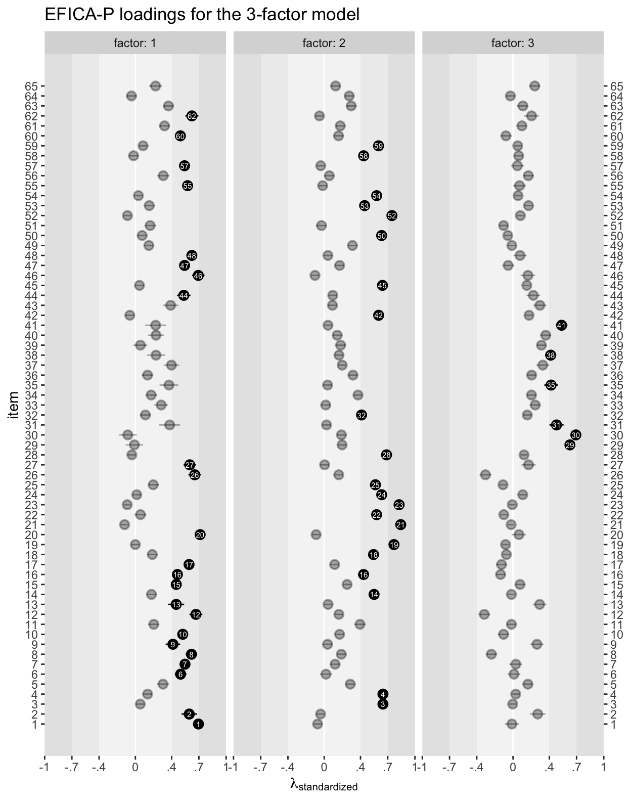
To reduce visual complexity, \(\lambda\)’s less than the conventional 0.4 threshold are semitransparent. Those above the threshold have the item number in the dot. I’m not going to offer an interpretation, here, since that’s not really the point of this post. But hopefully this will get you started fitting all the lavaan-based EFAs your heart desires.

How about ESEM?

If one can fit EFAs in lavaan, how about exploratory structural equation models (ESEM, Asparouhov & Muthén, 2009)? Yes, I believe one can. To get a sense, check out my search results at https://github.com/yrosseel/lavaan/search?q=esem. I haven’t had a reason to explore this for any of my projects, but it looks promising. If you master the lavaan ESEM method, maybe you could write a blog post of your own. Also, check out the blog post by Mateus Silvestrin, Exploratory Structural Equation Modeling in R.

Session information

sessionInfo()

## R version 4.2.0 (2022-04-22)
## Platform: x86_64-apple-darwin17.0 (64-bit)
## Running under: macOS Big Sur/Monterey 10.16
## 
## Matrix products: default
## BLAS:   /Library/Frameworks/R.framework/Versions/4.2/Resources/lib/libRblas.0.dylib
## LAPACK: /Library/Frameworks/R.framework/Versions/4.2/Resources/lib/libRlapack.dylib
## 
## locale:
## [1] en_US.UTF-8/en_US.UTF-8/en_US.UTF-8/C/en_US.UTF-8/en_US.UTF-8
## 
## attached base packages:
## [1] stats     graphics  grDevices utils     datasets  methods   base     
## 
## other attached packages:
##  [1] lavaan_0.6-12   forcats_0.5.1   stringr_1.4.1   dplyr_1.0.10    purrr_0.3.4     readr_2.1.2     tidyr_1.2.1    
##  [8] tibble_3.1.8    ggplot2_3.4.0   tidyverse_1.3.2
## 
## loaded via a namespace (and not attached):
##  [1] lubridate_1.8.0     assertthat_0.2.1    digest_0.6.30       utf8_1.2.2          R6_2.5.1           
##  [6] cellranger_1.1.0    backports_1.4.1     stats4_4.2.0        reprex_2.0.2        evaluate_0.18      
## [11] highr_0.9           httr_1.4.4          blogdown_1.15       pillar_1.8.1        rlang_1.0.6        
## [16] googlesheets4_1.0.1 readxl_1.4.1        rstudioapi_0.13     jquerylib_0.1.4     pbivnorm_0.6.0     
## [21] rmarkdown_2.16      labeling_0.4.2      googledrive_2.0.0   munsell_0.5.0       broom_1.0.1        
## [26] numDeriv_2016.8-1.1 compiler_4.2.0      modelr_0.1.8        xfun_0.35           pkgconfig_2.0.3    
## [31] mnormt_2.1.0        htmltools_0.5.3     tidyselect_1.1.2    bookdown_0.28       viridisLite_0.4.1  
## [36] fansi_1.0.3         crayon_1.5.2        tzdb_0.3.0          dbplyr_2.2.1        withr_2.5.0        
## [41] grid_4.2.0          jsonlite_1.8.3      gtable_0.3.1        lifecycle_1.0.3     DBI_1.1.3          
## [46] magrittr_2.0.3      scales_1.2.1        cli_3.4.1           stringi_1.7.8       cachem_1.0.6       
## [51] farver_2.1.1        fs_1.5.2            xml2_1.3.3          bslib_0.4.0         ellipsis_0.3.2     
## [56] generics_0.1.3      vctrs_0.5.0         tools_4.2.0         glue_1.6.2          hms_1.1.1          
## [61] fastmap_1.1.0       yaml_2.3.5          colorspace_2.0-3    gargle_1.2.0        rvest_1.0.2        
## [66] knitr_1.40          haven_2.5.1         sass_0.4.2

References

Arruda, M. A., Arruda, R., & Anunciação, L. (2020). Psychometric properties and clinical utility of the executive function inventory for children and adolescents: A large multistage populational study including children with ADHD. Applied Neuropsychology: Child, 1–17. https://doi.org/10.1080/21622965.2020.1726353
Asparouhov, T., & Muthén, B. (2009). Exploratory structural equation modeling. Structural Equation Modeling: A Multidisciplinary Journal, 16(3), 397–438. https://doi.org/10.1080/10705510903008204
Flora, D. B., & Curran, P. J. (2004). An empirical evaluation of alternative methods of estimation for confirmatory factor analysis with ordinal data. Psychological Methods, 9(4), 466. https://doi.org/10.1037/1082-989X.9.4.466
Li, C.-H. (2016). Confirmatory factor analysis with ordinal data: Comparing robust maximum likelihood and diagonally weighted least squares. Behavior Research Methods, 48(3), 936–949. https://doi.org/10.3758/s13428-015-0619-7
Revelle, W. (2022). psych: Procedures for psychological, psychometric, and personality research. https://CRAN.R-project.org/package=psych
Rosseel, Y. (2012). lavaan: An R package for structural equation modeling. Journal of Statistical Software, 48(2), 1–36. https://doi.org/10.18637/jss.v048.i02
Rosseel, Y., & Jorgensen, T. D. (2019). lavaan: Latent variable analysis [Manual]. https://lavaan.org
Sass, D. A., & Schmitt, T. A. (2010). A comparative investigation of rotation criteria within exploratory factor analysis. Multivariate Behavioral Research, 45(1), 73–103. https://doi.org/10.1080/00273170903504810
Schmitt, T. A. (2011). Current methodological considerations in exploratory and confirmatory factor analysis. Journal of Psychoeducational Assessment, 29(4), 304–321. https://doi.org/10.1177/0734282911406653
Wickham, H. (2022). tidyverse: Easily install and load the ’tidyverse’. https://CRAN.R-project.org/package=tidyverse
Wickham, H., Averick, M., Bryan, J., Chang, W., McGowan, L. D., François, R., Grolemund, G., Hayes, A., Henry, L., Hester, J., Kuhn, M., Pedersen, T. L., Miller, E., Bache, S. M., Müller, K., Ooms, J., Robinson, D., Seidel, D. P., Spinu, V., … Yutani, H. (2019). Welcome to the tidyverse. Journal of Open Source Software, 4(43), 1686. https://doi.org/10.21105/joss.01686
- Posted on:
- May 11, 2021
- Length:
- 11 minute read, 2321 words