Time-varying covariates in longitudinal multilevel models contain state- and trait-level information: This includes binary variables, too
By A. Solomon Kurz
October 31, 2019
tl;dr
When you have a time-varying covariate you’d like to add to a multilevel growth model, it’s important to break that variable into two. One part of the variable will account for within-person variation. The other part will account for between person variation. Keep reading to learn how you might do so when your time-varying covariate is binary.
I assume things.
For this post, I’m presuming you are familiar with longitudinal multilevel models and vaguely familiar with the basic differences between frequentist and Bayesian statistics. All code in is R, with a heavy use of the tidyverse–which you might learn a lot about here, especially chapter 5–, and the brms package for Bayesian regression.
Context
In my applied work, one of my collaborators collects longitudinal behavioral data. They are in the habit of analyzing their focal dependent variables (DVs) with variants of the longitudinal multilevel model, which is great. Though they often collect their primary independent variables (IVs) at all time points, they typically default to only using the baseline values for their IVs to predict the random intercepts and slopes of the focal DVs.
It seems like we’re making inefficient use of the data. At first I figured we’d just use the IVs at all time points, which would be treating them as time-varying covariates. But time varying covariates don’t allow one to predict variation in the random intercepts and slopes, which I and my collaborator would like to do. So while using the IVs at all time points as time-varying covariates makes use of more of the available data, it requires us to trade one substantive focus for another, which seems frustrating.
After low-key chewing on this for a while, I recalled that it’s possible to decompose time-varying covariates into measures of traits and states. Consider the simple case where your time-varying covariate, \(x_{ij}\) is continuous. In this notation, the \(x\) values vary across persons \(i\) and time points \(j\). If we compute the person level mean, \(\overline x_i\), that would be a time-invariant covariate and would, conceptually, be a measure of a person’s trait level for \(x\). Even if you do this, it’s still okay to include both \(\overline x_i\) and \(x_{ij}\) in the model equation. The former would be the time-invariant covariate that might predict the variation in the random intercepts and slopes. The latter would still serve as a time-varying covariate that might account for the within-person variation in the DV over time.
There, of course, are technicalities about how one might center \(\overline x_i\) and \(x_{ij}\) that one should carefully consider for these kinds of models.
Enders & Tofighi (2007) covered the issue from a cross-sectional perspective.
Hoffman (2015) covered it from a longitudinal perspective. But in the grand scheme of things, those are small potatoes. The main deal is that I can use our IVs as both time-varying and time-invariant predictors.
I was pretty excited once I remembered all this.
But then I realized that some of my collaborator’s IVs are binary, which initially seemed baffling, to me. Would it be sensible to compute \(\overline x_i\) for a binary time-varying covariate? What would that mean for the time-varying version of the variable? So I did what any responsible postdoctoral researcher would do. I posed the issue on Twitter.
Context: multilevel growth models.
— Solomon Kurz (@SolomonKurz) October 26, 2019
When you have a continuous time-varying covariate, you can decompose it into two variables, an id-level grand mean and the time-specific deviations from that mean. Is anyone aware of a complimentary approach for binary time-varying covariates?
My initial thoughts on the topic were a little confused. I wasn’t differentiating well between issues about the variance decomposition and centering and I’m a little embarrassed over that gaff. But I’m still glad I posed the question to Twitter. My virtual colleagues came through in spades! In particular, I’d like to give major shout outs to Andrea Howard ( @DrAndreaHoward), Mattan Ben-Shachar ( @mattansb), and Aidan Wright ( @aidangcw), who collectively pointed me to the solution. It was detailed in the references I listed, above: Enders & Tofighi (2007) and Hoffman (2015). Thank you, all!
Here’s the deal: Yes, you simply take the person-level means for the binary covariate \(x\). That will create a vector of time-invariant IVs ranging continuously from 0 to 1. They’ll be in a probability metric and they conceptually index a person’s probability of endorsing 1 over time. It’s basically the same as a batting average in baseball. You are at liberty to leave the time-invariant covariate in this metric, or you could center it by standardizing or some other sensible transformation. As for the state version of the IV, \(x_{ij}\), you’d just leave it exactly as it is. [There are other ways to code binary data, such as effects coding. I’m not a fan and will not be covering that in detail, here. But yes, you could recode your time-varying binary covariate that way, too.]
Break out the data
We should practice this with some data. I’ve been chipping away at working through Singer and Willett’s classic (2003) text, Applied longitudinal data analysis: Modeling change and event occurrence with brms and tidyverse code. You can find the working files in this GitHub repository. In chapter 5, Singer and Willett worked through a series of examples with a data set with a continuous DV and a binary IV. Here are those data.
library(tidyverse)

d <- read_csv("https://raw.githubusercontent.com/ASKurz/Applied-Longitudinal-Data-Analysis-with-brms-and-the-tidyverse/master/data/unemployment_pp.csv")

glimpse(d)
## Rows: 674
## Columns: 4
## $ id     <dbl> 103, 103, 103, 641, 641, 641, 741, 846, 846, 846, 937, 937, 111…
## $ months <dbl> 1.149897, 5.946612, 12.911704, 0.788501, 4.862423, 11.827515, 1…
## $ cesd   <dbl> 25, 16, 33, 27, 7, 25, 40, 2, 22, 0, 3, 8, 3, 0, 5, 7, 18, 26, …
## $ unemp  <dbl> 1, 1, 1, 1, 0, 0, 1, 1, 1, 0, 1, 0, 1, 1, 1, 1, 1, 0, 1, 0, 0, …
Set the stage with descriptive plots.
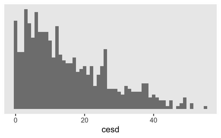
The focal DV is cesd, a continuous variable measuring depression. Singer and Willett (2003):
Each time participants completed the Center for Epidemiologic Studies’ Depression (CES-D) scale ( Radloff, 1977), which asks them to rate, on a four-point scale, the frequency with which they experience each of the 20 depressive symptoms. The CES-D scores can vary from a low or 0 for someone with no symptoms to a high of 80 for someone in serious distress. (p. 161)
Here’s what the cesd scores look like, collapsing over time.
theme_set(theme_gray() +
            theme(panel.grid = element_blank()))

d %>%
  ggplot(aes(x = cesd)) +
  geom_histogram(fill = "grey50", binwidth = 1) +
  scale_y_continuous(NULL, breaks = NULL)
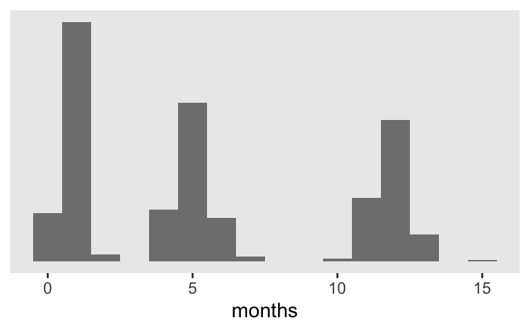
Since these are longutdnial data, our fundamental IV is a measure of time. That’s captured in the months column. Most participants have data on just three occasions and the months values range from about 0 to 15.
d %>%
  ggplot(aes(x = months)) +
  geom_histogram(fill = "grey50", binwidth = 1) +
  scale_y_continuous(NULL, breaks = NULL)
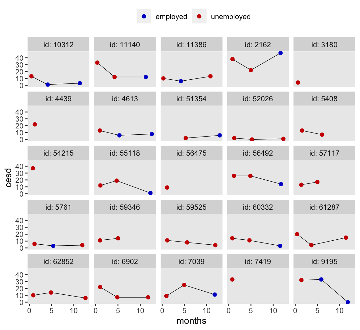
The main research question we’ll be addressing is: What do participants’ cesd scores look like over time and to what extent does their employment/unemployment status help explain their depression? So our substantive IV of interest is unemp, which is coded 0 = employed and 1 = unemployed. Since participants were recruited from local unemployment offices, everyone started off as unemp == 1. The values varied after that. Here’s a look at the data from a random sample of 25 of the participants.
# this makes `sample_n()` reproducible
set.seed(5)

# wrangle the data a little
d %>%
  nest(data = c(months, cesd, unemp)) %>%
  sample_n(size = 25) %>%
  unnest(data) %>%
  mutate(id = str_c("id: ", id),
         e  = if_else(unemp == 0, "employed", "unemployed")) %>%

  # plot
  ggplot(aes(x = months, y = cesd)) +
  geom_line(aes(group = id),
            size = 1/4) +
  geom_point(aes(color = e),
             size = 7/4) +
  scale_color_manual(NULL, values = c("blue3", "red3")) +
  theme(panel.grid      = element_blank(),
        legend.position = "top") +
  facet_wrap(~id, nrow = 5)
Embrace the hate.
To be honest, I kinda hate these data. There are too few measurement occasions within participants for my liking and the assessment schedule just seems bazar. As we’ll see in a bit, these data are also un-ideal to address exactly the kinds of models this blog is centered on.
Yet it’s for just these reasons I love these data. Real-world data analysis is ugly. The data are never what you want or expected them to be. So it seems the data we use in our educational materials should be equally terrible.
Much like we do for our most meaningful relationships, let’s embrace our hate/love ambivalence for our data with wide-open eyes and tender hearts. 🖤
Time to model.
Following Singer and Willett, we can define our first model using a level-1/level-2 specification. The level-1 model would be
$$\text{cesd}_{ij} = \pi_{0i} + \pi_{1i} \text{months}_{ij} + \pi_{2i} \text{unemp}_{ij} + \epsilon_{ij},$$
where \(\pi_{0i}\) is the intercept, \(\pi_{1i}\) is the effect of months on cesd, and \(\pi_{2i}\) is the effect of unemp on cesd. The final term, \(\epsilon_{ij}\), is the within-person variation not accounted for by the model–sometimes called error or residual variance. Our \(\epsilon_{ij}\) term follows the usual distribution of
$$ \epsilon_{ij} \sim \operatorname{Normal} (0, \sigma_\epsilon), $$
which, in words, means that the within-person variance estimates are normally distributed with a mean of zero and a standard deviation that’s estimated from the data. The corresponding level-2 model follows the form
$$
\begin{align*} \pi_{0i} & = \gamma_{00} + \zeta_{0i} \\ \pi_{1i} & = \gamma_{10} + \zeta_{1i} \\ \pi_{2i} & = \gamma_{20}, \end{align*}
$$
where \(\gamma_{00}\) is the grand mean for the intercept, which varies by person, as captured by the level-2 variance term \(\zeta_{0i}\). Similarly, \(\gamma_{10}\) is the grand mean for the effect of months, which varies by person, as captured by the second level-2 variance term \(\zeta_{1i}\). With this parameterization, it turns out \(\pi_{2i}\) does not vary by person and so its \(\gamma_{20}\) terms does not get a corresponding level-2 variance coefficient. If we wanted the effects of the time-varying covariate unemp to vary across individuals, we’d expand the definition of \(\pi_{2i}\) to be
$$ \pi_{2i} = \gamma_{20} + \zeta_{2i}. $$
Within our brms paradigm, the two level-2 variance parameters follow the form
$$
\begin{align*} \begin{bmatrix} \zeta_{0i} \\ \zeta_{1i} \\ \end{bmatrix} & \sim \operatorname{Normal} \left ( \begin{bmatrix} 0 \\ 0 \end{bmatrix}, \mathbf{D} \mathbf{\Omega} \mathbf{D}' \right ), \text{where} \\ \mathbf{D} & = \begin{bmatrix} \sigma_0 & 0 \\ 0 & \sigma_1 \end{bmatrix} \text{and} \\ \mathbf{\Omega} & = \begin{bmatrix} 1 & \rho_{01} \\ \rho_{01} & 1 \end{bmatrix}. \end{align*}
$$
I’ll be using a weakly-regularizing approach for the model priors in this post. I detail how I came to these in the
Chapter 5 file from my GitHub repo. If you check that file, you’ll see this model is a simplified version of fit10. Here are our priors:
$$
\begin{align*} \gamma_{00} & \sim \operatorname{Normal}(14.5, 20) \\ \gamma_{10}, \gamma_{20} & \sim \operatorname{Normal}(0, 10) \\ \sigma_\epsilon, \sigma_0, \sigma_1 & \sim \operatorname{Student-t}(3, 0, 10) \\ \Omega & \sim \operatorname{LKJ}(4). \end{align*}
$$
Feel free to explore different priors on your own. But now we’re done spelling our our first model, it’s time to fire up our main statistical package, brms.
library(brms)
We can fit the model with brms::brm(), like so.
fit1 <-
  brm(data = d,
      family = gaussian,
      cesd ~ 0 + intercept + months + unemp + (1 + months | id),
      prior = c(prior(normal(14.5, 20), class = b, coef = "intercept"),
                prior(normal(0, 10),    class = b),
                prior(student_t(3, 0, 10), class = sd),
                prior(student_t(3, 0, 10), class = sigma),
                prior(lkj(4), class = cor)),
      iter = 2000, warmup = 1000, chains = 4, cores = 4,
      control = list(adapt_delta = .95),
      seed = 5)
Before we explore the results from this model, we should point out that we only included unemp as a level-1 time-varying predictor. As Hoffman pointed out in her (2015) text, the flaw in this approach is that
time-varying predictors contain both between-person and within-person information…
[Thus,] time-varying predictors will need to be represented by two separate predictors that distinguish their between-person and within-person sources of variance in order to properly distinguish their potential between-person and within-person effects on a longitudinal outcome. (pp. 329, 333, emphasis in the original)
The simplest way to separate the between-person variance in unemp from the pure within-person variation is to compute a new variable capturing \(\overline{\text{unemp}}_i\), the person-level means for their unemployment status. Here we compute that variable, which we’ll call unemp_id_mu.
d <-
  d %>%
  group_by(id) %>%
  mutate(unemp_id_mu = mean(unemp)) %>%
  ungroup()

head(d)
## # A tibble: 6 × 5
##      id months  cesd unemp unemp_id_mu
##   <dbl>  <dbl> <dbl> <dbl>       <dbl>
## 1   103  1.15     25     1       1
## 2   103  5.95     16     1       1
## 3   103 12.9      33     1       1
## 4   641  0.789    27     1       0.333
## 5   641  4.86      7     0       0.333
## 6   641 11.8      25     0       0.333
Because umemp is binary, \(\overline{\text{unemp}}_i\) can only take on values ranging from 0 to 1. Here are the unique values we have for unemp_id_mu.
d %>%
  distinct(unemp_id_mu)
## # A tibble: 4 × 1
##   unemp_id_mu
##         <dbl>
## 1       1
## 2       0.333
## 3       0.667
## 4       0.5
Because each participant’s \(\overline{\text{unemp}}_i\) was based on 3 or fewer measurement occasions, basic algebra limited the variability in our unemp_id_mu values. You’ll also note that there were no 0s. This, recall, is because participants were recruited at local unemployment offices, leaving all participants with at least one starting value of unemp == 1.
We should rehearse how we might interpret the unemp_id_mu values. First recall they are considered level-2 variables; they are between-participant variables. Since they are averages of binary data, they are in a probability metric. In this instance, they are each participants overall probability of being unemployed–their trait-level propensity toward unemployment. No doubt these values would be more reliable if they were computed from data on a greater number of assessment occasions. But with three measurement occasions, we at least have a sense of stability.
Since our new \(\overline{\text{unemp}}_i\) variable is a level-2 predictor, the level-1 equation for our next model is the same as before:
$$\text{cesd}_{ij} = \pi_{0i} + \pi_{1i} \text{months}_{ij} + \pi_{2i} \text{unemp}_{ij} + \epsilon_{ij}.$$
However, there are two new terms in our level-2 model,
$$
\begin{align*} \pi_{0i} & = \gamma_{00} + \gamma_{01} (\overline{\text{unemp}}_i) + \zeta_{0i} \\ \pi_{1i} & = \gamma_{10} + \gamma_{11} (\overline{\text{unemp}}_i) + \zeta_{1i} \\ \pi_{2i} & = \gamma_{20}, \end{align*}
$$
which is meant to convey that \(\overline{\text{unemp}}_i\) is allowed to explain variability in both initial status on CES-D scores (i.e., the random intercepts) and change in CES-D scores over time (i.e., the random months slopes). Our variance parameters are all the same:
$$
\begin{align*} \epsilon_{ij} & \sim \operatorname{Normal} (0, \sigma_\epsilon) \text{ and} \\ \begin{bmatrix} \zeta_{0i} \\ \zeta_{1i} \\ \end{bmatrix} & \sim \operatorname{Normal} \left ( \begin{bmatrix} 0 \\ 0 \end{bmatrix}, \mathbf{D} \mathbf{\Omega} \mathbf{D}' \right ), \text{where} \\ \mathbf{D} & = \begin{bmatrix} \sigma_0 & 0 \\ 0 & \sigma_1 \end{bmatrix} \text{and} \\ \mathbf{\Omega} & = \begin{bmatrix} 1 & \rho_{01} \\ \rho_{01} & 1 \end{bmatrix}. \end{align*}
$$
Our priors also follow the same basic specification as before:
$$
\begin{align*} \gamma_{00} & \sim \operatorname{Normal}(14.5, 20) \\ \gamma_{01}, \gamma_{10}, \gamma_{11}, \gamma_{20} & \sim \operatorname{Normal}(0, 10) \\ \sigma_\epsilon, \sigma_0, \sigma_1 & \sim \operatorname{Student-t}(3, 0, 10) \\ \Omega & \sim \operatorname{LKJ}(4). \end{align*}
$$
Note, however, that the inclusion of our new level-2 predictor, \((\overline{\text{unemp}}_i)\), changes the meaning of the intercept, \(\gamma_{00}\). The intercept is now the expected value for a person for whom unemp_id_mu == 0 at the start of the study (i.e., months == 0). I still think our intercept prior from the first model is fine for this example. But do think carefully about the priors you use in your real-world data analyses.
Here’s how to fit the udpdate model with brms.
fit2 <-
  brm(data = d,
      family = gaussian,
      cesd ~ 0 + intercept + months + unemp + unemp_id_mu + unemp_id_mu:months + (1 + months | id),
      prior = c(prior(normal(14.5, 20), class = b, coef = "intercept"),
                prior(normal(0, 10),    class = b),
                prior(student_t(3, 0, 10), class = sd),
                prior(student_t(3, 0, 10), class = sigma),
                prior(lkj(4), class = cor)),
      iter = 2000, warmup = 1000, chains = 4, cores = 4,
      seed = 5)
We should fit one more model before we look at the parameters. If you were paying close attention, above, you may have noticed how it’s odd that we kept unemp_id_mu in it’s natural metric. Sure, it’s fine in principle–sensible even–to use a variable in a probability metric. But in this particular study, none of the participants had a value of unemp_id_mu == 0 because all of them were unemployed at the first time point. Though it is mathematically kosher to fit a model with an intercept based on unemp_id_mu == 0, it’s awkward to interpret. So in this case, it makes sense to transform the metric of our level-2 predictor. Perhaps the simplest way is to standardize the variable. That would then give an intercept based on the average unemp_id_mu value and a \(\gamma_{01}\) coefficient that was the expected change in intercept based on a one-standard-deviation higher value in unemp_id_mu. Let’s compute that new standardized variable, which we’ll call unemp_id_mu_s.
d <-
  d %>%
  nest(data = c(months:unemp)) %>%
  mutate(unemp_id_mu_s = (unemp_id_mu - mean(unemp_id_mu)) / sd(unemp_id_mu)) %>%
  unnest(data)

head(d)
## # A tibble: 6 × 6
##      id unemp_id_mu months  cesd unemp unemp_id_mu_s
##   <dbl>       <dbl>  <dbl> <dbl> <dbl>         <dbl>
## 1   103       1      1.15     25     1         0.873
## 2   103       1      5.95     16     1         0.873
## 3   103       1     12.9      33     1         0.873
## 4   641       0.333  0.789    27     1        -1.58
## 5   641       0.333  4.86      7     0        -1.58
## 6   641       0.333 11.8      25     0        -1.58
The model formula is the same as before with the exception that we replace unemp_id_mu with unemp_id_mu_s. For simplicity, I’m leaving the priors the way they were.
fit3 <-
  brm(data = d,
      family = gaussian,
      cesd ~ 0 + intercept + months + unemp + unemp_id_mu_s + unemp_id_mu_s:months + (1 + months | id),
      prior = c(prior(normal(14.5, 20), class = b, coef = "intercept"),
                prior(normal(0, 10),    class = b),
                prior(student_t(3, 0, 10), class = sd),
                prior(student_t(3, 0, 10), class = sigma),
                prior(lkj(4), class = cor)),
      iter = 2000, warmup = 1000, chains = 4, cores = 4,
      control = list(adapt_delta = .9),
      seed = 5)
Instead of examining each of the model summaries one by one, we’ll condense the information into a series of coefficient plots. For simplicity, we’ll restrict our focus to the \(\gamma\) parameters.
# extract the `fit1` summaries
fixef(fit1) %>%
  data.frame() %>%
  rownames_to_column("par") %>%
  mutate(fit = "fit1") %>%
  bind_rows(
    # add the `fit2` summaries
    fixef(fit2) %>%
      data.frame() %>%
      rownames_to_column("par") %>%
      mutate(fit = "fit2"),
    # add the `fit2` summaries
    fixef(fit3) %>%
      data.frame() %>%
      rownames_to_column("par") %>%
      mutate(fit = "fit3")
  ) %>%
  # rename the parameters
  mutate(gamma = case_when(
    par == "intercept"     ~ "gamma[0][0]",
    par == "months"        ~ "gamma[1][0]",
    par == "unemp"         ~ "gamma[2][0]",
    str_detect(par, ":")   ~ "gamma[1][1]",
    par == "unemp_id_mu"   ~ "gamma[0][1]",
    par == "unemp_id_mu_s" ~ "gamma[0][1]"
  )) %>%

  # plot!
  ggplot(aes(x = fit, y = Estimate, ymin = Q2.5, ymax = Q97.5)) +
  geom_hline(yintercept = 0, color = "white") +
  geom_pointrange(fatten = 3) +
  xlab(NULL) +
  coord_flip() +
  facet_wrap(~ gamma, nrow = 3, scale = "free_x", labeller = label_parsed)
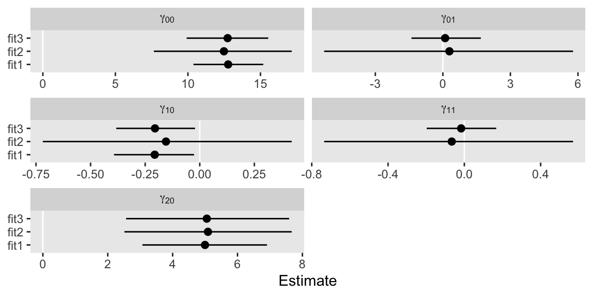
In case you’re not familiar with the output from the brms::fixef() function, each of the parameter estimates are summarized by their posterior means (i.e,. the dots) and percentile-based 95% intervals (i.e., the horizontal lines).
Recall how earlier I complained that these data weren’t particularly good for demonstrating this method? Well, here you finally get to see why. Regardless of the model, the estimates didn’t change much. In these data, the predictive utility of our between-level variable, unemp_id_mu–standardized or not–, was just about zilch. This is summarized by the \(\gamma_{01}\) and \(\gamma_{11}\) parameters. Both are centered around zero for both models containing them. Thus adding in an inconsequential level-2 predictor had little effect on its level-1 companion, unemp, which was expressed by \(\gamma_{20}\).
Depressing as these results are, the practice was still worthwhile. Had we not decomposed our time-varying unemp variable into its within- and between-level components, we would never had known that the trait levels of umemp were inconsequential for these analyses. Now we know. For these models, all the action for unemp was at the within-person level.
This is also the explanation for why we focused on the \(\gamma\)s to the neglect of the variance parameters. Because our unemp_id_mu variables were poor predictors of the random effects, there was no reason to expect they’d differ meaningfully across models. And because unemp_id_mu is only a level-2 predictor, it never had any hope for changing the estimates for \(\sigma_\epsilon\).
What about centering umemp?
If you look through our primary two references for this post, Enders & Tofighi (2007) and Hoffman (2015), you’ll see both works spend a lot of time on discussing how one might center the level-1 versions of the time-varying covariates. If unemp was a continuous variable, we would have had to contend with that issue, too. But this just isn’t necessary with binary variables. They have a sensible interpretation when left in the typical 0/1 format. So my recommendation is when you’re decomposing your binary time-varying covariates, put your focus on meaningfully centering the level-2 version of the variable. Leave the level-1 version alone. However, if you’re really interested in playing around with alternatives like effects coding, Enders and Tofighi provided several recommendations.
Session info
sessionInfo()
## R version 4.3.0 (2023-04-21)
## Platform: aarch64-apple-darwin20 (64-bit)
## Running under: macOS Ventura 13.4
##
## Matrix products: default
## BLAS:   /Library/Frameworks/R.framework/Versions/4.3-arm64/Resources/lib/libRblas.0.dylib
## LAPACK: /Library/Frameworks/R.framework/Versions/4.3-arm64/Resources/lib/libRlapack.dylib;  LAPACK version 3.11.0
##
## locale:
## [1] en_US.UTF-8/en_US.UTF-8/en_US.UTF-8/C/en_US.UTF-8/en_US.UTF-8
##
## time zone: America/Chicago
## tzcode source: internal
##
## attached base packages:
## [1] stats     graphics  grDevices utils     datasets  methods   base
##
## other attached packages:
##  [1] brms_2.19.0     Rcpp_1.0.10     lubridate_1.9.2 forcats_1.0.0
##  [5] stringr_1.5.0   dplyr_1.1.2     purrr_1.0.1     readr_2.1.4
##  [9] tidyr_1.3.0     tibble_3.2.1    ggplot2_3.4.2   tidyverse_2.0.0
##
## loaded via a namespace (and not attached):
##   [1] tensorA_0.36.2       rstudioapi_0.14      jsonlite_1.8.5
##   [4] magrittr_2.0.3       TH.data_1.1-2        estimability_1.4.1
##   [7] farver_2.1.1         nloptr_2.0.3         rmarkdown_2.22
##  [10] vctrs_0.6.3          minqa_1.2.5          base64enc_0.1-3
##  [13] blogdown_1.17        htmltools_0.5.5      distributional_0.3.2
##  [16] curl_5.0.1           sass_0.4.6           StanHeaders_2.26.27
##  [19] bslib_0.5.0          htmlwidgets_1.6.2    plyr_1.8.8
##  [22] sandwich_3.0-2       emmeans_1.8.6        zoo_1.8-12
##  [25] cachem_1.0.8         igraph_1.4.3         mime_0.12
##  [28] lifecycle_1.0.3      pkgconfig_2.0.3      colourpicker_1.2.0
##  [31] Matrix_1.5-4         R6_2.5.1             fastmap_1.1.1
##  [34] shiny_1.7.4          digest_0.6.31        colorspace_2.1-0
##  [37] ps_1.7.5             crosstalk_1.2.0      projpred_2.6.0
##  [40] labeling_0.4.2       fansi_1.0.4          timechange_0.2.0
##  [43] abind_1.4-5          mgcv_1.8-42          compiler_4.3.0
##  [46] bit64_4.0.5          withr_2.5.0          backports_1.4.1
##  [49] inline_0.3.19        shinystan_2.6.0      gamm4_0.2-6
##  [52] pkgbuild_1.4.1       highr_0.10           MASS_7.3-58.4
##  [55] gtools_3.9.4         loo_2.6.0            tools_4.3.0
##  [58] httpuv_1.6.11        threejs_0.3.3        glue_1.6.2
##  [61] callr_3.7.3          nlme_3.1-162         promises_1.2.0.1
##  [64] grid_4.3.0           checkmate_2.2.0      reshape2_1.4.4
##  [67] generics_0.1.3       gtable_0.3.3         tzdb_0.4.0
##  [70] hms_1.1.3            utf8_1.2.3           pillar_1.9.0
##  [73] markdown_1.7         vroom_1.6.3          posterior_1.4.1
##  [76] later_1.3.1          splines_4.3.0        lattice_0.21-8
##  [79] survival_3.5-5       bit_4.0.5            tidyselect_1.2.0
##  [82] miniUI_0.1.1.1       knitr_1.43           gridExtra_2.3
##  [85] bookdown_0.34        stats4_4.3.0         xfun_0.39
##  [88] bridgesampling_1.1-2 matrixStats_1.0.0    DT_0.28
##  [91] rstan_2.21.8         stringi_1.7.12       yaml_2.3.7
##  [94] boot_1.3-28.1        evaluate_0.21        codetools_0.2-19
##  [97] emo_0.0.0.9000       cli_3.6.1            RcppParallel_5.1.7
## [100] shinythemes_1.2.0    xtable_1.8-4         munsell_0.5.0
## [103] processx_3.8.1       jquerylib_0.1.4      coda_0.19-4
## [106] parallel_4.3.0       rstantools_2.3.1     ellipsis_0.3.2
## [109] assertthat_0.2.1     prettyunits_1.1.1    dygraphs_1.1.1.6
## [112] bayesplot_1.10.0     Brobdingnag_1.2-9    lme4_1.1-33
## [115] mvtnorm_1.2-2        scales_1.2.1         xts_0.13.1
## [118] crayon_1.5.2         rlang_1.1.1          multcomp_1.4-24
## [121] shinyjs_2.1.0
- Posted on:
- October 31, 2019
- Length:
- 19 minute read, 3859 words
- Tags:
- Bayesian brms multilevel R tutorial