Bayesian power analysis: Part III.b. What about 0/1 data?

Version 1.2.0

Edited on December 11, 2022, to use the new as_draws_df() workflow.

Orientation

In the last post, we covered how the Poisson distribution is handy for modeling count data. Binary data are even weirder than counts. They typically only take on two values: 0 and 1. Sometimes 0 is a stand-in for “no” and 1 for “yes” (e.g., Are you an expert in Bayesian power analysis? For me that would be 0). You can also have data of this kind if you asked people whether they’d like to choose option A or B. With those kinds of data, you might arbitrarily code A as 0 and B as 1. Binary data also often stand in for trials where 0 = “fail” and 1 = “success.” For example, if you answered “Yes” to the question Are all data normally distributed? we’d mark your answer down as a 0.

Though 0’s and 1’s are popular, sometimes binary data appear in their aggregated form. Let’s say I gave you 10 algebra questions and you got 7 of them right. Here’s one way to encode those data.

n <- 10
z <- 7

rep(0:1, times = c(n - z, z))

##  [1] 0 0 0 1 1 1 1 1 1 1

In that example, n stood for the total number of trials and z was the number you got correct (i.e., the number of times we encoded your response as a 1). A more compact way to encode that data is with two columns, one for z and the other for n.

library(tidyverse)

tibble(z = z,
       n = n)

## # A tibble: 1 × 2
##       z     n
##   <dbl> <dbl>
## 1     7    10

So then if you gave those same 10 questions to four of your friends, we could encode the results like this.

set.seed(3)

tibble(id = letters[1:5],
       z  = rpois(n = 5, lambda = 5),
       n  = n)

## # A tibble: 5 × 3
##   id        z     n
##   <chr> <int> <dbl>
## 1 a         3    10
## 2 b         7    10
## 3 c         4    10
## 4 d         4    10
## 5 e         5    10

If you were b, you’d be the smart one in the group.

Anyway, whether working with binary or aggregated binary data, we’re interested in the probability a given trial will be 1.

Logistic regression with unaggregated binary data

Taking unaggregated binary data as a starting point, given \(d\) data that includes a variable \(y\) where the value in the \(i^\text{th}\) row is a 0 or a 1, we’d like to know the probability a given trial would be 1, given \(d\) [i.e., \(p(y_i = 1 | d)\)]. The binomial distribution will help us get that estimate for \(p\). We’ll do so within the context of a logistic regression model following the form

$$ \begin{align*} y_i & \sim \text{Binomial} (n = 1, p_i) \\ \operatorname{logit} (p_i) & = \beta_0, \end{align*} $$

were the logit function is defined as the log odds

$$ \operatorname{logit} (p_i) = \log \left (\frac{p_i}{1 - p_i} \right ), $$

which also means that

$$ \log \left (\frac{p_i}{1 - p_i} \right ) = \beta_0. $$

In those formulas, \(\beta_0\) is the intercept. In a binomial model with no predictors¹, the intercept \(\beta_0\) is just the estimate for \(p\), but in the log-odds metric. So yes, similar to the Poisson models from the last post, we typically use a link function with our binomial models. Instead of the log link, we use the logit because it constrains the posterior for \(p\) to values between 0 and 1. Just as the null value for a probability is .5, the null value for the parameters within a logistic regression model is typically 0.

As with the Poisson, I’m not going to go into a full-blown tutorial on the binomial distribution or on logistic regression. For more thorough introductions, check out chapters 9 through 10 in McElreath’s ( 2015) Statistical rethinking or Agresti’s ( 2015) Foundations of linear and generalized linear models.

We need data.

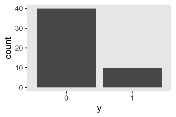
Time to simulate some data. Let’s say we’d like to estimate the probability someone will hit a ball in a baseball game. Nowadays, batting averages for professional baseball players tend around .25 (see here). So if we wanted to simulate 50 at-bats, we might do so like this.

set.seed(3)

d <- tibble(y = rbinom(n = 50, size = 1, prob = .25))

str(d)

## tibble [50 × 1] (S3: tbl_df/tbl/data.frame)
##  $ y: int [1:50] 0 1 0 0 0 0 0 0 0 0 ...

Here are what those data look like in a bar plot.

theme_set(theme_gray() + theme(panel.grid = element_blank()))

d %>% 
  mutate(y = factor(y)) %>% 
  
  ggplot(aes(x = y)) +
  geom_bar()

Time to model.

To practice modeling those data, we’ll want to fire up the brms package ( Bürkner, 2017, 2018, 2022).

library(brms)

We can use the get_prior() function to get the brms default for our intercept-only logistic regression model.

get_prior(data = d, 
          family = binomial,
          y | trials(1) ~ 1)

## Intercept ~ student_t(3, 0, 2.5)

As it turns out, that’s a really liberal prior. We might step up a bit and put a more skeptical normal(0, 2) prior on that intercept. With the context of our logit link, that still puts a 95% probability that the \(p\) is between .02 and .98, which is almost the entire parameter space. Here’s how to fit the model with the brm() function.

fit1 <-
  brm(data = d, 
      family = binomial,
      y | trials(1) ~ 1,
      prior(normal(0, 2), class = Intercept),
      seed = 3)

In the brm() formula syntax, including a | bar on the left side of a formula indicates we have extra supplementary information about our criterion variable. In this case, that information is that each y value corresponds to a single trial [i.e., trials(1)], which itself corresponds to the \(n = 1\) portion of the statistical formula, above. Here are the results.

print(fit1)

##  Family: binomial 
##   Links: mu = logit 
## Formula: y | trials(1) ~ 1 
##    Data: d (Number of observations: 50) 
##   Draws: 4 chains, each with iter = 2000; warmup = 1000; thin = 1;
##          total post-warmup draws = 4000
## 
## Population-Level Effects: 
##           Estimate Est.Error l-95% CI u-95% CI Rhat Bulk_ESS Tail_ESS
## Intercept    -1.39      0.36    -2.10    -0.73 1.00     1327     1362
## 
## Draws were sampled using sampling(NUTS). For each parameter, Bulk_ESS
## and Tail_ESS are effective sample size measures, and Rhat is the potential
## scale reduction factor on split chains (at convergence, Rhat = 1).

Remember that that intercept is on the scale of the logit link, the log odds. We can transform it with the brms::inv_logit_scaled() function.

fixef(fit1)["Intercept", 1] %>% 
  inv_logit_scaled()

## [1] 0.1992104

If we’d like to view the full posterior distribution, we’ll need to work with the posterior draws themselves. Then we’ll plot.

# extract the posterior draws
as_draws_df(fit1) %>% 
  # transform from the log-odds to a probability metric
  transmute(p = inv_logit_scaled(b_Intercept)) %>% 
  
  # plot!
  ggplot(aes(x = p)) +
  geom_density(fill = "grey25", size = 0) +
  scale_x_continuous("probability of a hit", limits = c(0, 1)) +
  scale_y_continuous(NULL, breaks = NULL)

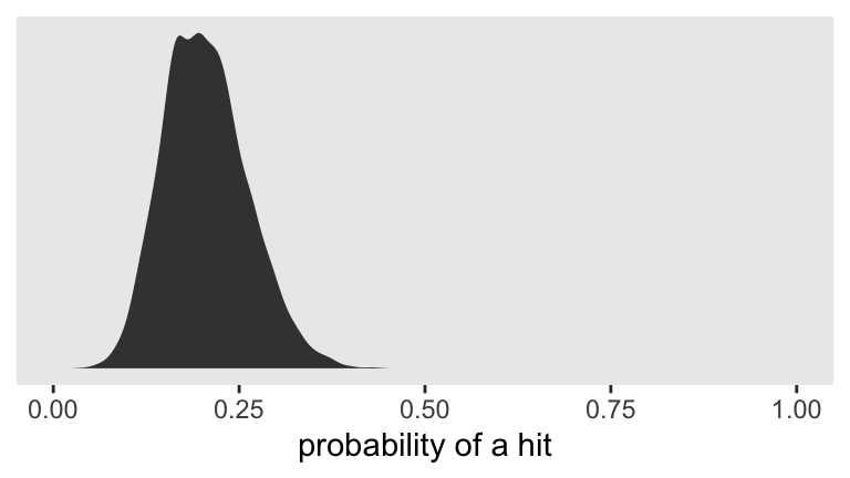
Looks like the null hypothesis of \(p = .5\) is not credible for this simulation. If we’d like the posterior median and percentile-based 95% intervals, we might use the median_qi() function from the handy tidybayes package ( Kay, 2022).

library(tidybayes)

as_draws_df(fit1) %>% 
  transmute(p = inv_logit_scaled(b_Intercept)) %>% 
  median_qi()

## # A tibble: 1 × 6
##       p .lower .upper .width .point .interval
##   <dbl>  <dbl>  <dbl>  <dbl> <chr>  <chr>    
## 1 0.201  0.109  0.325   0.95 median qi

Yep, .5 was not within those intervals.

But what about power?

That’s enough preliminary work. Let’s see what happens when we do a mini power analysis with 100 iterations. First we set up our simulation function using the same methods we introduced in earlier blog posts.

sim_data_fit <- function(seed, n_player) {
  
  n_trials <- 1
  prob_hit <- .25
  
  set.seed(seed)
  
  d <- tibble(y = rbinom(n    = n_player, 
                         size = n_trials, 
                         prob = prob_hit))
  
  update(fit1,
         newdata = d,
         seed = seed) %>% 
    as_draws_df() %>% 
    transmute(p = inv_logit_scaled(b_Intercept)) %>% 
    median_qi() %>% 
    select(.lower:.upper)
  
}

Simulate.

sim1 <-
  tibble(seed = 1:100) %>% 
  mutate(ci = map(seed, sim_data_fit, n_player = 50)) %>% 
  unnest(ci)

You might plot the intervals.

sim1 %>% 
  ggplot(aes(x = seed, ymin = .lower, ymax = .upper)) +
  geom_hline(yintercept = c(.25, .5), color = "white") +
  geom_linerange() +
  xlab("seed (i.e., simulation index)") +
  scale_y_continuous("probability of hitting the ball", limits = c(0, 1))

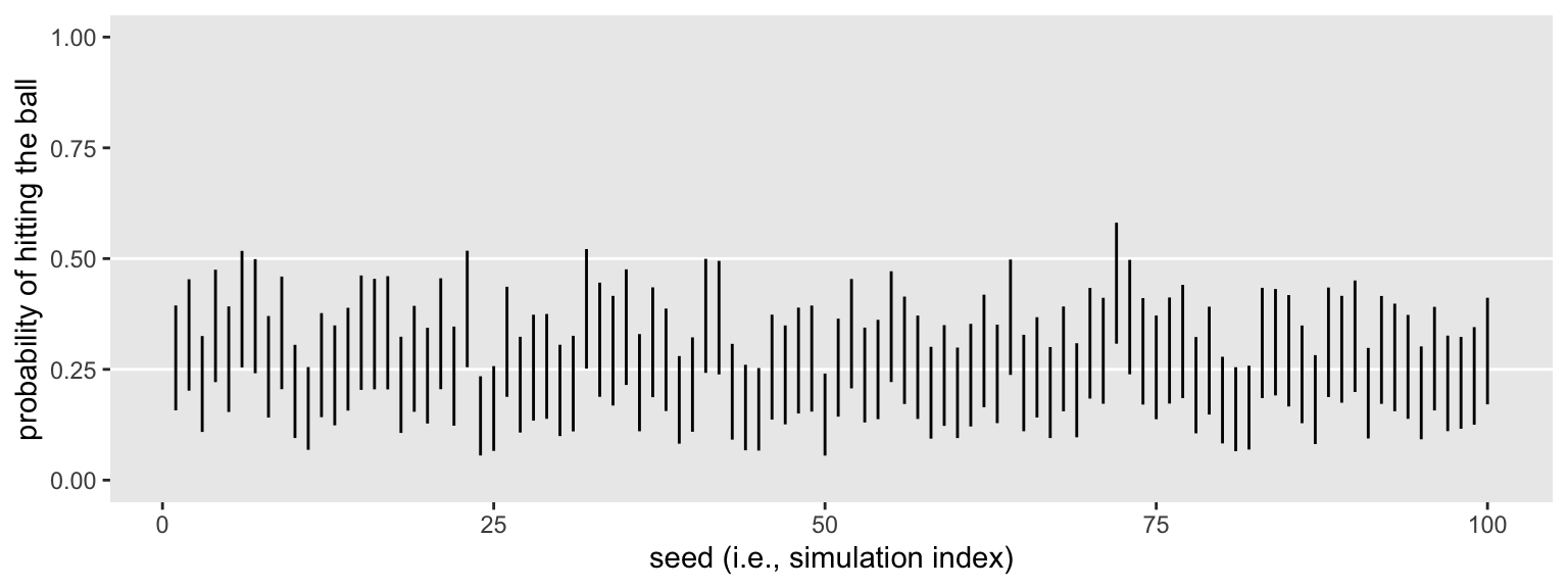
Like one of my old coworkers used to say: Purtier ’n a hog! Here we’ll summarize the results both in terms of their conventional power, their mean width, and the proportion of widths more narrow than .25. Why .25? I don’t know. Without a substantively-informed alternative, it’s as good a criterion as any.

sim1 %>% 
  mutate(width = .upper - .lower) %>% 
  summarise(`conventional power` = mean(.upper < .5),
            `mean width`         = mean(width),
            `width below .25`    = mean(width < .25))

## # A tibble: 1 × 3
##   `conventional power` `mean width` `width below .25`
##                  <dbl>        <dbl>             <dbl>
## 1                 0.96        0.231              0.78

Depending on your study needs, you’d adjust your sample size accordingly, do a mini simulation or two first, and then follow up with a proper power simulation with 1000+ iterations.

I should point out that whereas in the last post we evaluated the power of the Poisson model with the parameters on the scale of the link function, here we evaluated the power for our logistic regression model after transforming the intercept back into the probability metric. Both methods are fine. I recommend you run your power simulation based on how you want to interpret and report your results.

We should also acknowledge that this was our first example of a power simulation that wasn’t based on some group comparison. Comparing groups is fine and normal and important. And it’s also the case that we can care about power and/or parameter precision for more than group-based analyses. Our simulation-based approach is fine for both.

Aggregated binomial regression

It’s no more difficult to simulate and work with aggregated binomial data. But since the mechanics for brms::brm() and thus the down-the-road simulation setup are a little different, we should practice. With our new setup, we’ll consider a new example. Since .25 is the typical batting average, it might better sense to define the null hypothesis like this:

$$H_0 \text{: } p = .25.$$

Consider a case where we had some intervention where we expected a new batting average of .35. How many trials would we need, then, to either reject \(H_0\) or perhaps estimate \(p\) with a satisfactory degree of precision? Here’s what the statistical formula for the implied aggregated binomial model might look like:

$$ \begin{align*} y_i & \sim \text{Binomial} (n, p_i) \\ \operatorname{logit} (p_i) & = \beta_0. \end{align*} $$

The big change is we no longer defined \(n\) as 1. Let’s say we wanted our aggregated binomial data set to contain the summary statistics for \(n = 100\) trials. Here’s what that might look like.

n_trials <- 100
prob_hit <- .35

set.seed(3)

d <- tibble(n_trials = n_trials,
            y = rbinom(n    = 1, 
                       size = n_trials, 
                       prob = prob_hit))

d

## # A tibble: 1 × 2
##   n_trials     y
##      <dbl> <int>
## 1      100    32

Now we have two columns. The first, n_trials, indicates how many cases or trials we’re summarizing. The second, y, indicates how many successes/1’s/hits we might expect given \(p = .35\). This is the aggregated binomial equivalent of if we had a 100-row vector composed of 32 1’s and 68 0’s.

Now, before we discuss fitting the model with brms, let’s talk priors. Since we’ve updated our definition of \(H_0\), it might make sense to update the prior for \(\beta_0\). As it turns out, setting that prior to normal(-1, 0.5) puts the posterior mode at about .25 on the probability space, but with fairly wide 95% intervals ranging from about .12 to .5. Though centered on our updated null value, this prior is still quite permissive given our hypothesized \(p = .35\). Let’s give it a whirl.

To fit an aggregated binomial model with the brm() function, we augment the <criterion> | trials() syntax where the value that goes in trials() is either a fixed number or variable in the data indexing \(n\). Our approach will be the latter.

fit2 <-
  brm(data = d, 
      family = binomial,
      y | trials(n_trials) ~ 1,
      prior(normal(-1, 0.5), class = Intercept),
      seed = 3)

Inspect the summary.

print(fit2)

##  Family: binomial 
##   Links: mu = logit 
## Formula: y | trials(n_trials) ~ 1 
##    Data: d (Number of observations: 1) 
##   Draws: 4 chains, each with iter = 2000; warmup = 1000; thin = 1;
##          total post-warmup draws = 4000
## 
## Population-Level Effects: 
##           Estimate Est.Error l-95% CI u-95% CI Rhat Bulk_ESS Tail_ESS
## Intercept    -0.80      0.20    -1.19    -0.42 1.00     1524     1697
## 
## Draws were sampled using sampling(NUTS). For each parameter, Bulk_ESS
## and Tail_ESS are effective sample size measures, and Rhat is the potential
## scale reduction factor on split chains (at convergence, Rhat = 1).

After a transformation, here’s what that looks like in a plot.

as_draws_df(fit2) %>% 
  transmute(p = inv_logit_scaled(b_Intercept)) %>% 
  
  ggplot(aes(x = p, y = 0)) +
  stat_halfeye(.width = c(.5, .95)) +
  scale_x_continuous("probability of a hit", limits = c(0, 1)) +
  scale_y_continuous(NULL, breaks = NULL)

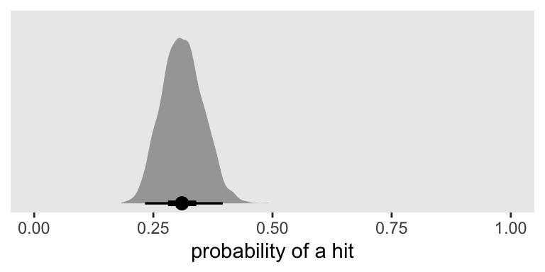
Based on a single simulation, it looks like \(n = 100\) won’t quite be enough to reject \(H_0 \text{: } p = .25\) with a conventional 2-sided 95% interval. But it does look like we’re in the ballpark and that our basic data + model setup will work for a larger-scale simulation. Here’s an example of how you might update our custom simulation function.

sim_data_fit <- function(seed, n_trials) {
  
  prob_hit <- .35
  
  set.seed(seed)
  
  d <- tibble(y = rbinom(n    = 1, 
                         size = n_trials, 
                         prob = prob_hit),
              n_trials = n_trials)
  
  update(fit2,
         newdata = d,
         seed = seed) %>% 
    as_draws_df() %>% 
    transmute(p = inv_logit_scaled(b_Intercept)) %>% 
    median_qi() %>% 
    select(.lower:.upper)
  
}

Simulate, this time trying out \(n = 120\).

sim2 <-
  tibble(seed = 1:100) %>% 
  mutate(ci = map(seed, sim_data_fit, n_trials = 120)) %>% 
  unnest(ci)

Plot the intervals.

sim2 %>% 
  ggplot(aes(x = seed, ymin = .lower, ymax = .upper)) +
  geom_hline(yintercept = c(.25, .35), color = "white") +
  geom_linerange() +
  xlab("seed (i.e., simulation index)") +
  scale_y_continuous("probability of hitting the ball",
                     limits = c(0, 1), breaks = c(0, .25, .35, 1))

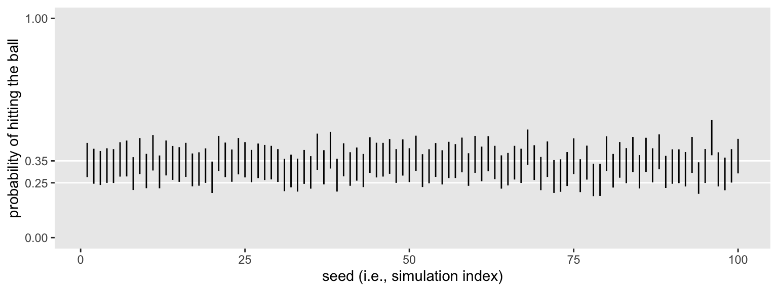
Overall, those intervals look pretty good. They’re fairly narrow and are hovering around the data generating \(p = .35\). But many are still crossing the .25 threshold. Let’s see the results of a formal summary.

sim2 %>% 
  mutate(width = .upper - .lower) %>% 
  summarise(`conventional power` = mean(.lower > .25),
            `mean width`         = mean(width),
            `width below .2`     = mean(width < .2))

## # A tibble: 1 × 3
##   `conventional power` `mean width` `width below .2`
##                  <dbl>        <dbl>            <dbl>
## 1                 0.54        0.155                1

All widths were narrower than .2 and the mean width was about .16. In the abstract that might seem reasonably precise. But we’re still not precise enough to reject \(H_0\) with a conventional power level. Depending on your needs, adjust the \(n\) accordingly and simulate again.

Now you’ve got a sense of how to work with the binomial likelihood for (aggregated)binary data, next time we’ll play with Likert-type data.

Session info

sessionInfo()

## R version 4.2.0 (2022-04-22)
## Platform: x86_64-apple-darwin17.0 (64-bit)
## Running under: macOS Big Sur/Monterey 10.16
## 
## Matrix products: default
## BLAS:   /Library/Frameworks/R.framework/Versions/4.2/Resources/lib/libRblas.0.dylib
## LAPACK: /Library/Frameworks/R.framework/Versions/4.2/Resources/lib/libRlapack.dylib
## 
## locale:
## [1] en_US.UTF-8/en_US.UTF-8/en_US.UTF-8/C/en_US.UTF-8/en_US.UTF-8
## 
## attached base packages:
## [1] stats     graphics  grDevices utils     datasets  methods   base     
## 
## other attached packages:
##  [1] tidybayes_3.0.2 brms_2.18.0     Rcpp_1.0.9      forcats_0.5.1  
##  [5] stringr_1.4.1   dplyr_1.0.10    purrr_0.3.4     readr_2.1.2    
##  [9] tidyr_1.2.1     tibble_3.1.8    ggplot2_3.4.0   tidyverse_1.3.2
## 
## loaded via a namespace (and not attached):
##   [1] readxl_1.4.1         backports_1.4.1      plyr_1.8.7          
##   [4] igraph_1.3.4         svUnit_1.0.6         splines_4.2.0       
##   [7] crosstalk_1.2.0      TH.data_1.1-1        rstantools_2.2.0    
##  [10] inline_0.3.19        digest_0.6.30        htmltools_0.5.3     
##  [13] fansi_1.0.3          magrittr_2.0.3       checkmate_2.1.0     
##  [16] googlesheets4_1.0.1  tzdb_0.3.0           modelr_0.1.8        
##  [19] RcppParallel_5.1.5   matrixStats_0.62.0   xts_0.12.1          
##  [22] sandwich_3.0-2       prettyunits_1.1.1    colorspace_2.0-3    
##  [25] rvest_1.0.2          ggdist_3.2.0         haven_2.5.1         
##  [28] xfun_0.35            callr_3.7.3          crayon_1.5.2        
##  [31] jsonlite_1.8.3       lme4_1.1-31          survival_3.4-0      
##  [34] zoo_1.8-10           glue_1.6.2           gtable_0.3.1        
##  [37] gargle_1.2.0         emmeans_1.8.0        distributional_0.3.1
##  [40] pkgbuild_1.3.1       rstan_2.21.7         abind_1.4-5         
##  [43] scales_1.2.1         mvtnorm_1.1-3        DBI_1.1.3           
##  [46] miniUI_0.1.1.1       xtable_1.8-4         stats4_4.2.0        
##  [49] StanHeaders_2.21.0-7 DT_0.24              htmlwidgets_1.5.4   
##  [52] httr_1.4.4           threejs_0.3.3        arrayhelpers_1.1-0  
##  [55] posterior_1.3.1      ellipsis_0.3.2       pkgconfig_2.0.3     
##  [58] loo_2.5.1            farver_2.1.1         sass_0.4.2          
##  [61] dbplyr_2.2.1         utf8_1.2.2           labeling_0.4.2      
##  [64] tidyselect_1.1.2     rlang_1.0.6          reshape2_1.4.4      
##  [67] later_1.3.0          munsell_0.5.0        cellranger_1.1.0    
##  [70] tools_4.2.0          cachem_1.0.6         cli_3.4.1           
##  [73] generics_0.1.3       broom_1.0.1          ggridges_0.5.3      
##  [76] evaluate_0.18        fastmap_1.1.0        yaml_2.3.5          
##  [79] processx_3.8.0       knitr_1.40           fs_1.5.2            
##  [82] nlme_3.1-159         mime_0.12            projpred_2.2.1      
##  [85] xml2_1.3.3           compiler_4.2.0       bayesplot_1.9.0     
##  [88] shinythemes_1.2.0    rstudioapi_0.13      gamm4_0.2-6         
##  [91] reprex_2.0.2         bslib_0.4.0          stringi_1.7.8       
##  [94] highr_0.9            ps_1.7.2             blogdown_1.15       
##  [97] Brobdingnag_1.2-8    lattice_0.20-45      Matrix_1.4-1        
## [100] nloptr_2.0.3         markdown_1.1         shinyjs_2.1.0       
## [103] tensorA_0.36.2       vctrs_0.5.0          pillar_1.8.1        
## [106] lifecycle_1.0.3      jquerylib_0.1.4      bridgesampling_1.1-2
## [109] estimability_1.4.1   httpuv_1.6.5         R6_2.5.1            
## [112] bookdown_0.28        promises_1.2.0.1     gridExtra_2.3       
## [115] codetools_0.2-18     boot_1.3-28          colourpicker_1.1.1  
## [118] MASS_7.3-58.1        gtools_3.9.3         assertthat_0.2.1    
## [121] withr_2.5.0          shinystan_2.6.0      multcomp_1.4-20     
## [124] mgcv_1.8-40          parallel_4.2.0       hms_1.1.1           
## [127] grid_4.2.0           coda_0.19-4          minqa_1.2.5         
## [130] rmarkdown_2.16       googledrive_2.0.0    shiny_1.7.2         
## [133] lubridate_1.8.0      base64enc_0.1-3      dygraphs_1.1.1.6

References

Agresti, A. (2015). Foundations of linear and generalized linear models. John Wiley & Sons. https://www.wiley.com/en-us/Foundations+of+Linear+and+Generalized+Linear+Models-p-9781118730034
Bürkner, P.-C. (2017). brms: An R package for Bayesian multilevel models using Stan. Journal of Statistical Software, 80(1), 1–28. https://doi.org/10.18637/jss.v080.i01
Bürkner, P.-C. (2018). Advanced Bayesian multilevel modeling with the R package brms. The R Journal, 10(1), 395–411. https://doi.org/10.32614/RJ-2018-017
Bürkner, P.-C. (2022). brms: Bayesian regression models using ’Stan’. https://CRAN.R-project.org/package=brms
Kay, M. (2022). tidybayes: Tidy data and ’geoms’ for Bayesian models. https://CRAN.R-project.org/package=tidybayes
McElreath, R. (2015). Statistical rethinking: A Bayesian course with examples in R and Stan. CRC press. https://xcelab.net/rm/statistical-rethinking/
-
In case this is all new to you and you and you had the question in your mind: Yes, you can add predictors to the logistic regression model. Say we had a model with two predictors,
\(x_1\)and\(x_2\). Our statistical model would then follow the form\(\operatorname{logit} (p_i) = \beta_0 + \beta_1 x_{1i} + \beta_2 x_{2i}\). ↩︎
- Posted on:
- August 27, 2019
- Length:
- 15 minute read, 3010 words