Bayesian meta-analysis in brms
By A. Solomon Kurz
October 14, 2018
[edited Dec 10, 2022]
Preamble
I released the first bookdown version of my Statistical Rethinking with brms, ggplot2, and the tidyverse project a couple weeks ago. I consider it the 0.9.0 version1. I wanted a little time to step back from the project before giving it a final edit for the first major edition. I also wanted to give others a little time to take a look and suggest edits, which some thankfully have.
Now some time has passed, it’s become clear I’d like to add a bonus section on Bayesian meta-analysis. IMO, this is a natural extension of the hierarchical models McElreath introduced in chapter’s 12 and 13 of his text and of the measurement-error models he introduced in chapter 14. So the purpose of this post is to present a rough draft of how I’d like to introduce fitting meta-analyses with Bürkner’s great brms package.
I intend to tack this section onto the end of chapter 14. If you have any constrictive criticisms, please pass them along.
Here’s the rough draft (which I updated on 2018-11-12):
Rough draft: Meta-analysis
If your mind isn’t fully blown by those measurement-error and missing-data models, let’s keep building. As it turns out, meta-analyses are often just special kinds of multilevel measurement-error models. Thus, you can use brms::brm() to fit Bayesian meta-analyses, too.
Before we proceed, I should acknowledge that this section is heavily influenced by Matti Vourre’s great blog post, Meta-analysis is a special case of Bayesian multilevel modeling. And since McElreath’s text doesn’t directly address meta-analyses, we’ll take further inspiration from Gelman, Carlin, Stern, Dunson, Vehtari, and Rubin’s Bayesian data analysis, Third edition. We’ll let Gelman and colleagues introduce the topic:
Discussions of meta-analysis are sometimes imprecise about the estimands of interest in the analysis, especially when the primary focus is on testing the null hypothesis of no effect in any of the studies to be combined. Our focus is on estimating meaningful parameters, and for this objective there appear to be three possibilities, accepting the overarching assumption that the studies are comparable in some broad sense. The first possibility is that we view the studies as identical replications of each other, in the sense we regard the individuals in all the studies as independent samples from a common population, with the same outcome measures and so on. A second possibility is that the studies are so different that the results of any one study provide no information about the results of any of the others. A third, more general, possibility is that we regard the studies as exchangeable but not necessarily either identical or completely unrelated; in other words we allow differences from study to study, but such that the differences are not expected a priori to have predictable effects favoring one study over another.… This third possibility represents a continuum between the two extremes, and it is this exchangeable model (with unknown hyperparameters characterizing the population distribution) that forms the basis of our Bayesian analysis…
The first potential estimand of a meta-analysis, or a hierarchically structured problem in general, is the mean of the distribution of effect sizes, since this represents the overall ‘average’ effect across all studies that could be regarded as exchangeable with the observed studies. Other possible estimands are the effect size in any of the observed studies and the effect size in another, comparable (exchangeable) unobserved study. (pp. 125–126, emphasis in the original)
The basic version of a Bayesian meta-analysis follows the form
$$y_i \sim \text{Normal}(\theta_i, \sigma_i)$$
where \(y_i\) = the point estimate for the effect size of a single study, \(i\), which is presumed to have been a draw from a Normal distribution centered on \(\theta_i\). The data in meta-analyses are typically statistical summaries from individual studies. The one clear lesson from this chapter is that those estimates themselves come with error and those errors should be fully expressed in the meta-analytic model. Which we do. The standard error from study \(i\) is specified \(\sigma_i\), which is also a stand-in for the standard deviation of the Normal distribution from which the point estimate was drawn. Do note, we’re not estimating \(\sigma_i\), here. Those values we take directly from the original studies.
Building on the model, we further presume that study \(i\) is itself just one draw from a population of related studies, each of which have their own effect sizes. As such. we presume \(\theta_i\) itself has a distribution following the form
$$\theta_i \sim \text{Normal} (\mu, \tau)$$
where \(\mu\) is the meta-analytic effect (i.e., the population mean) and \(\tau\) is the variation around that mean, what you might also think of as \(\sigma_\tau\).
Since there’s no example of a meta-analysis in the text, we’ll have to look elsewhere. We’ll focus on Gershoff and Grogan-Kaylor’s (2016) paper, Spanking and Child Outcomes: Old Controversies and New Meta-Analyses. From their introduction, we read:
Around the world, most children (80%) are spanked or otherwise physically punished by their parents ( UNICEF, 2014). The question of whether parents should spank their children to correct misbehaviors sits at a nexus of arguments from ethical, religious, and human rights perspectives both in the U.S. and around the world ( Gershoff, 2013). Several hundred studies have been conducted on the associations between parents’ use of spanking or physical punishment and children’s behavioral, emotional, cognitive, and physical outcomes, making spanking one of the most studied aspects of parenting. What has been learned from these hundreds of studies? (p. 453)
Our goal will be to learn Bayesian meta-analysis by answering part of that question. I’ve transcribed the values directly from Gershoff and Grogan-Kaylor’s paper and saved them as a file called spank.xlsx.
You can find the data in
this project’s GitHub repository. Let’s load them and glimpse().
spank <- readxl::read_excel("spank.xlsx")

library(tidyverse)
glimpse(spank)
## Rows: 111
## Columns: 8
## $ study   <chr> "Bean and Roberts (1981)", "Day and Roberts (1983)", "Minton, …
## $ year    <dbl> 1981, 1983, 1971, 1988, 1990, 1961, 1962, 1990, 2002, 2005, 19…
## $ outcome <chr> "Immediate defiance", "Immediate defiance", "Immediate defianc…
## $ between <dbl> 1, 1, 0, 1, 1, 0, 1, 0, 0, 0, 1, 0, 1, 0, 0, 0, 0, 1, 0, 0, 0,…
## $ within  <dbl> 0, 0, 1, 0, 0, 1, 0, 1, 1, 1, 0, 1, 0, 1, 1, 1, 1, 0, 1, 1, 1,…
## $ d       <dbl> -0.74, 0.36, 0.34, -0.08, 0.10, 0.63, 0.19, 0.47, 0.14, -0.18,…
## $ ll      <dbl> -1.76, -1.04, -0.09, -1.01, -0.82, 0.16, -0.14, 0.20, -0.42, -…
## $ ul      <dbl> 0.28, 1.77, 0.76, 0.84, 1.03, 1.10, 0.53, 0.74, 0.70, 0.13, 2.…
In this paper, the effect size of interest is a Cohen’s d, derived from the formula
$$d = \frac{\mu_\text{treatment} - \mu_\text{comparison}}{\sigma_\text{pooled}}$$
where
$$\sigma_\text{pooled} = \sqrt{\frac{((n_1 - 1) \sigma_1^2) + ((n_2 - 1) \sigma_2^2)}{n_1 + n_2 -2}}$$
To help make the equation for \(d\) clearer for our example, we might re-express it as
$$d = \frac{\mu_\text{spanked} - \mu_\text{not spanked}}{\sigma_{pooled}}$$
McElreath didn’t really focus on effect sizes in his text. If you need a refresher, you might check out Kelley and Preacher’s On effect size. But in words, Cohen’s d is a standardized mean difference between two groups.
So if you look back up at the results of glimpse(spank), you’ll notice the column d, which is indeed a vector of Cohen’s d effect sizes. The last two columns, ll and ul are the lower and upper limits of the associated 95% frequentist confidence intervals. But we don’t want confidence intervals for our d-values; we want their standard errors. Fortunately, we can compute those with the following formula
$$\textit{SE} = \frac{\text{upper limit } – \text{lower limit}}{3.92}$$
Here it is in code.
spank <-
  spank %>%
  mutate(se = (ul - ll) / 3.92)

glimpse(spank)
## Rows: 111
## Columns: 9
## $ study   <chr> "Bean and Roberts (1981)", "Day and Roberts (1983)", "Minton, …
## $ year    <dbl> 1981, 1983, 1971, 1988, 1990, 1961, 1962, 1990, 2002, 2005, 19…
## $ outcome <chr> "Immediate defiance", "Immediate defiance", "Immediate defianc…
## $ between <dbl> 1, 1, 0, 1, 1, 0, 1, 0, 0, 0, 1, 0, 1, 0, 0, 0, 0, 1, 0, 0, 0,…
## $ within  <dbl> 0, 0, 1, 0, 0, 1, 0, 1, 1, 1, 0, 1, 0, 1, 1, 1, 1, 0, 1, 1, 1,…
## $ d       <dbl> -0.74, 0.36, 0.34, -0.08, 0.10, 0.63, 0.19, 0.47, 0.14, -0.18,…
## $ ll      <dbl> -1.76, -1.04, -0.09, -1.01, -0.82, 0.16, -0.14, 0.20, -0.42, -…
## $ ul      <dbl> 0.28, 1.77, 0.76, 0.84, 1.03, 1.10, 0.53, 0.74, 0.70, 0.13, 2.…
## $ se      <dbl> 0.52040816, 0.71683673, 0.21683673, 0.47193878, 0.47193878, 0.…
Now our data are ready, we can express our first Bayesian meta-analysis with the formula
$$
\begin{eqnarray} \text{d}_i & \sim & \text{Normal}(\theta_i, \sigma_i = \text{se}_i) \\ \theta_i & \sim & \text{Normal} (\mu, \tau) \\ \mu & \sim & \text{Normal} (0, 1) \\ \tau & \sim & \text{HalfCauchy} (0, 1) \end{eqnarray}
$$
The last two lines, of course, spell out our priors. In psychology, it’s pretty rare to see Cohen’s d-values greater than the absolute value of \(\pm 1\). So in the absence of more specific domain knowledge–which I don’t have–, it seems like \(\text{Normal} (0, 1)\) is a reasonable place to start. And just like McElreath used \(\text{HalfCauchy} (0, 1)\) as the default prior for the group-level standard deviations,
it makes sense to use it here for our meta-analytic \(\tau\) parameter.
Let’s load brms.
library(brms)
Here’s the code for the first model.
b14.5 <-
  brm(data = spank, family = gaussian,
      d | se(se) ~ 1 + (1 | study),
      prior = c(prior(normal(0, 1), class = Intercept),
                prior(cauchy(0, 1), class = sd)),
      iter = 2000, warmup = 1000, cores = 4, chains = 4,
      seed = 14)
One thing you might notice is our se(se) function excluded the sigma argument. If you recall from section 14.1, we specified sigma = T in our measurement-error models. The brms default is that within se(), sigma = FALSE. As such, we have no estimate for sigma the way we would if we were doing this analysis with the raw data from the studies. Hopefully this makes sense. The uncertainty around the d-value for each study \(i\) has already been encoded in the data as se.
This brings us to another point. We typically perform meta-analyses on data summaries. In my field and perhaps in yours, this is due to the historical accident that it has not been the norm among researchers to make their data publicly available. So effect size summaries were the best we typically had. However, times are changing (e.g.,
here,
here). If the raw data from all the studies for your meta-analysis are available, you can just fit a multilevel model in which the data are nested in the studies. Heck, you could even allow the studies to vary by \(\sigma\) by taking the
distributional modeling approach and specify something like sigma ~ 0 + study or even sigma ~ 1 + (1 | study).
But enough technical talk. Let’s look at the model results.
print(b14.5)
##  Family: gaussian
##   Links: mu = identity; sigma = identity
## Formula: d | se(se) ~ 1 + (1 | study)
##    Data: spank (Number of observations: 111)
##   Draws: 4 chains, each with iter = 2000; warmup = 1000; thin = 1;
##          total post-warmup draws = 4000
##
## Group-Level Effects:
## ~study (Number of levels: 76)
##               Estimate Est.Error l-95% CI u-95% CI Rhat Bulk_ESS Tail_ESS
## sd(Intercept)     0.26      0.03     0.21     0.33 1.00      806     1429
##
## Population-Level Effects:
##           Estimate Est.Error l-95% CI u-95% CI Rhat Bulk_ESS Tail_ESS
## Intercept     0.37      0.03     0.30     0.44 1.01      496      955
##
## Family Specific Parameters:
##       Estimate Est.Error l-95% CI u-95% CI Rhat Bulk_ESS Tail_ESS
## sigma     0.00      0.00     0.00     0.00   NA       NA       NA
##
## Draws were sampled using sampling(NUTS). For each parameter, Bulk_ESS
## and Tail_ESS are effective sample size measures, and Rhat is the potential
## scale reduction factor on split chains (at convergence, Rhat = 1).
Thus, in our simple Bayesian meta-analysis, we have a population Cohen’s d of about 0.37. Our estimate for \(\tau\), 0.26, suggests we have quite a bit of between-study variability. One question you might ask is: What exactly are these Cohen’s ds measuring, anyways? We’ve encoded that in the outcome vector of the spank data.
spank %>%
  distinct(outcome) %>%
  knitr::kable()
| outcome |
|---|
| Immediate defiance |
| Low moral internalization |
| Child aggression |
| Child antisocial behavior |
| Child externalizing behavior problems |
| Child internalizing behavior problems |
| Child mental health problems |
| Child alcohol or substance abuse |
| Negative parent–child relationship |
| Impaired cognitive ability |
| Low self-esteem |
| Low self-regulation |
| Victim of physical abuse |
| Adult antisocial behavior |
| Adult mental health problems |
| Adult alcohol or substance abuse |
| Adult support for physical punishment |
There are a few things to note. First, with the possible exception of Adult support for physical punishment, all of the outcomes are negative. We prefer conditions associated with lower values for things like Child aggression and Adult mental health problems. Second, the way the data are coded, larger effect sizes are interpreted as more negative outcomes associated with children having been spanked. That is, our analysis suggests spanking children is associated with worse outcomes. What might not be immediately apparent is that even though there are 111 cases in the data, there are only 76 distinct studies.
spank %>%
  distinct(study) %>%
  count()
## # A tibble: 1 × 1
##       n
##   <int>
## 1    76
In other words, some studies have multiple outcomes. In order to better accommodate the study- and outcome-level variances, let’s fit a cross-classified Bayesian meta-analysis reminiscent of the cross-classified chimp model from Chapter 13.
b14.6 <-
  brm(data = spank, family = gaussian,
      d | se(se) ~ 1 + (1 | study) + (1 | outcome),
      prior = c(prior(normal(0, 1), class = Intercept),
                prior(cauchy(0, 1), class = sd)),
      iter = 2000, warmup = 1000, cores = 4, chains = 4,
      seed = 14)
print(b14.6)
##  Family: gaussian
##   Links: mu = identity; sigma = identity
## Formula: d | se(se) ~ 1 + (1 | study) + (1 | outcome)
##    Data: spank (Number of observations: 111)
##   Draws: 4 chains, each with iter = 2000; warmup = 1000; thin = 1;
##          total post-warmup draws = 4000
##
## Group-Level Effects:
## ~outcome (Number of levels: 17)
##               Estimate Est.Error l-95% CI u-95% CI Rhat Bulk_ESS Tail_ESS
## sd(Intercept)     0.08      0.03     0.04     0.15 1.00      947     1728
##
## ~study (Number of levels: 76)
##               Estimate Est.Error l-95% CI u-95% CI Rhat Bulk_ESS Tail_ESS
## sd(Intercept)     0.25      0.03     0.20     0.32 1.00      809     1703
##
## Population-Level Effects:
##           Estimate Est.Error l-95% CI u-95% CI Rhat Bulk_ESS Tail_ESS
## Intercept     0.35      0.04     0.27     0.43 1.00      867     1454
##
## Family Specific Parameters:
##       Estimate Est.Error l-95% CI u-95% CI Rhat Bulk_ESS Tail_ESS
## sigma     0.00      0.00     0.00     0.00   NA       NA       NA
##
## Draws were sampled using sampling(NUTS). For each parameter, Bulk_ESS
## and Tail_ESS are effective sample size measures, and Rhat is the potential
## scale reduction factor on split chains (at convergence, Rhat = 1).
Now we have two \(\tau\) parameters. We might plot them to get a sense of where the variance is at.
as_draws_df(b14.6) %>%
  select(starts_with("sd")) %>%
  gather(key, tau) %>%
  mutate(key = str_remove(key, "sd_") %>% str_remove(., "__Intercept")) %>%

  ggplot(aes(x = tau, fill = key)) +
  geom_density(color = "transparent", alpha = 2/3) +
  scale_fill_viridis_d(NULL, end = .85) +
  scale_y_continuous(NULL, breaks = NULL) +
  xlab(expression(tau)) +
  theme(panel.grid = element_blank())
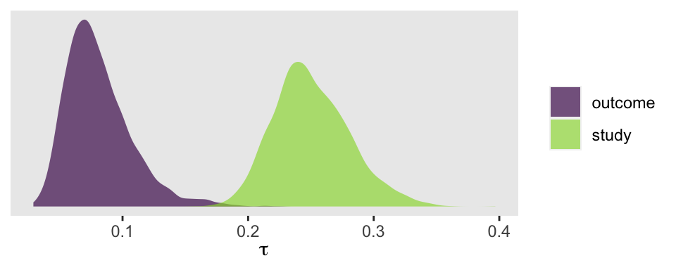
So at this point, the big story is there’s more variability between the studies than there is the outcomes. But I still want to get a sense of the individual outcomes. Here we’ll use tidybayes::stat_halfeye() to help us make our version of a
forest plot.
# load tidybayes
library(tidybayes)

b14.6 %>%
  spread_draws(b_Intercept, r_outcome[outcome,]) %>%
  # add the grand mean to the group-specific deviations
  mutate(mu = b_Intercept + r_outcome) %>%
  ungroup() %>%
  mutate(outcome = str_replace_all(outcome, "[.]", " ")) %>%

  # plot
  ggplot(aes(x = mu, y = reorder(outcome, mu))) +
  geom_vline(xintercept = fixef(b14.6)[1, 1], color = "white", size = 1) +
  geom_vline(xintercept = fixef(b14.6)[1, 3:4], color = "white", linetype = 2) +
  stat_halfeye(.width = .95, size = 2/3) +
  labs(x = expression(italic("Cohen's d")),
       y = NULL) +
  theme(panel.grid   = element_blank(),
        axis.ticks.y = element_blank(),
        axis.text.y  = element_text(hjust = 0))
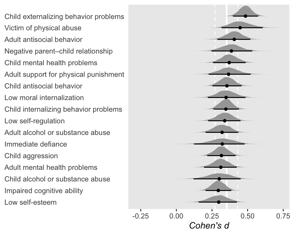
The solid and dashed vertical white lines in the background mark off the grand mean (i.e., the meta-analytic effect) and its 95% intervals. But anyway, there’s not a lot of variability across the outcomes. Let’s go one step further with the model. Doubling back to Gelman and colleagues, we read:
When assuming exchangeability we assume there are no important covariates that might form the basis of a more complex model, and this assumption (perhaps misguidedly) is widely adopted in meta-analysis. What if other information (in addition to the data
\((n, y)\)) is available to distinguish among the\(J\)studies in a meta-analysis, so that an exchangeable model is inappropriate? In this situation, we can expand the framework of the model to be exchangeable in the observed data and covariates, for example using a hierarchical regression model. (p. 126)
One important covariate Gershoff and Grogan-Kaylor addressed in their meta-analysis was the type of study. The 76 papers they based their meta-analysis on contained both between- and within-participants designs. In the spank data, we’ve dummy coded that information with the between and within vectors. Both are dummy variables and within = 1 - between. Here are the counts.
spank %>%
  count(between)
## # A tibble: 2 × 2
##   between     n
##     <dbl> <int>
## 1       0    71
## 2       1    40
When I use dummies in my models, I prefer to have the majority group stand as the reference category. As such, I typically name those variables by the minority group. In this case, most occasions are based on within-participant designs. Thus, we’ll go ahead and add the between variable to the model. While we’re at it, we’ll practice using the 0 + intercept syntax.
b14.7 <-
  brm(data = spank, family = gaussian,
      d | se(se) ~ 0 + intercept + between + (1 | study) + (1 | outcome),
      prior = c(prior(normal(0, 1), class = b),
                prior(cauchy(0, 1), class = sd)),
      iter = 2000, warmup = 1000, cores = 4, chains = 4,
      seed = 14)
print(b14.7)
##  Family: gaussian
##   Links: mu = identity; sigma = identity
## Formula: d | se(se) ~ 0 + intercept + between + (1 | study) + (1 | outcome)
##    Data: spank (Number of observations: 111)
##   Draws: 4 chains, each with iter = 2000; warmup = 1000; thin = 1;
##          total post-warmup draws = 4000
##
## Group-Level Effects:
## ~outcome (Number of levels: 17)
##               Estimate Est.Error l-95% CI u-95% CI Rhat Bulk_ESS Tail_ESS
## sd(Intercept)     0.08      0.03     0.04     0.14 1.00     1639     2402
##
## ~study (Number of levels: 76)
##               Estimate Est.Error l-95% CI u-95% CI Rhat Bulk_ESS Tail_ESS
## sd(Intercept)     0.25      0.03     0.20     0.32 1.01      933     1506
##
## Population-Level Effects:
##           Estimate Est.Error l-95% CI u-95% CI Rhat Bulk_ESS Tail_ESS
## intercept     0.38      0.05     0.28     0.48 1.00     1154     1739
## between      -0.07      0.07    -0.21     0.07 1.00     1088     1841
##
## Family Specific Parameters:
##       Estimate Est.Error l-95% CI u-95% CI Rhat Bulk_ESS Tail_ESS
## sigma     0.00      0.00     0.00     0.00   NA       NA       NA
##
## Draws were sampled using sampling(NUTS). For each parameter, Bulk_ESS
## and Tail_ESS are effective sample size measures, and Rhat is the potential
## scale reduction factor on split chains (at convergence, Rhat = 1).
Let’s take a closer look at b_between.
as_draws_df(b14.7) %>%

  ggplot(aes(x = b_between, y = 0)) +
  stat_halfeye(point_interval = median_qi, .width = c(.5, .95)) +
  labs(x = "Overall difference for between- vs within-participant designs",
       y = NULL) +
  scale_y_continuous(NULL, breaks = NULL) +
  theme(panel.grid = element_blank())
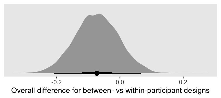
That difference isn’t as large I’d expect it to be. But then again, I’m no spanking researcher. So what do I know?
There are other things you might do with these data. For example, you might check for trends by year or, as the authors did in their manuscript, distinguish among different severities of corporal punishment. But I think we’ve gone far enough to get you started.
If you’d like to learn more about these methods, do check out Vourre’s
Meta-analysis is a special case of Bayesian multilevel modeling. From his blog, you’ll learn additional tricks, like making a more traditional-looking forest plot with the brmstools::forest() function and how our Bayesian brms method compares with frequentist meta-analyses via the
metafor package. You might also check out Williams, Rast, and Bürkner’s manuscript,
Bayesian Meta-Analysis with Weakly Informative Prior Distributions to give you an empirical justification for using a half-Cauchy prior for your meta-analysis \(\tau\) parameters.
Session info
sessionInfo()
## R version 4.2.0 (2022-04-22)
## Platform: x86_64-apple-darwin17.0 (64-bit)
## Running under: macOS Big Sur/Monterey 10.16
##
## Matrix products: default
## BLAS:   /Library/Frameworks/R.framework/Versions/4.2/Resources/lib/libRblas.0.dylib
## LAPACK: /Library/Frameworks/R.framework/Versions/4.2/Resources/lib/libRlapack.dylib
##
## locale:
## [1] en_US.UTF-8/en_US.UTF-8/en_US.UTF-8/C/en_US.UTF-8/en_US.UTF-8
##
## attached base packages:
## [1] stats     graphics  grDevices utils     datasets  methods   base
##
## other attached packages:
##  [1] tidybayes_3.0.2 brms_2.18.0     Rcpp_1.0.9      forcats_0.5.1
##  [5] stringr_1.4.1   dplyr_1.0.10    purrr_0.3.4     readr_2.1.2
##  [9] tidyr_1.2.1     tibble_3.1.8    ggplot2_3.4.0   tidyverse_1.3.2
##
## loaded via a namespace (and not attached):
##   [1] readxl_1.4.1         backports_1.4.1      plyr_1.8.7
##   [4] igraph_1.3.4         svUnit_1.0.6         splines_4.2.0
##   [7] crosstalk_1.2.0      TH.data_1.1-1        rstantools_2.2.0
##  [10] inline_0.3.19        digest_0.6.30        htmltools_0.5.3
##  [13] fansi_1.0.3          magrittr_2.0.3       checkmate_2.1.0
##  [16] googlesheets4_1.0.1  tzdb_0.3.0           modelr_0.1.8
##  [19] RcppParallel_5.1.5   matrixStats_0.62.0   xts_0.12.1
##  [22] sandwich_3.0-2       prettyunits_1.1.1    colorspace_2.0-3
##  [25] rvest_1.0.2          ggdist_3.2.0         haven_2.5.1
##  [28] xfun_0.35            callr_3.7.3          crayon_1.5.2
##  [31] jsonlite_1.8.3       lme4_1.1-31          survival_3.4-0
##  [34] zoo_1.8-10           glue_1.6.2           gtable_0.3.1
##  [37] gargle_1.2.0         emmeans_1.8.0        distributional_0.3.1
##  [40] pkgbuild_1.3.1       rstan_2.21.7         abind_1.4-5
##  [43] scales_1.2.1         mvtnorm_1.1-3        DBI_1.1.3
##  [46] miniUI_0.1.1.1       viridisLite_0.4.1    xtable_1.8-4
##  [49] stats4_4.2.0         StanHeaders_2.21.0-7 DT_0.24
##  [52] htmlwidgets_1.5.4    httr_1.4.4           threejs_0.3.3
##  [55] arrayhelpers_1.1-0   posterior_1.3.1      ellipsis_0.3.2
##  [58] pkgconfig_2.0.3      loo_2.5.1            farver_2.1.1
##  [61] sass_0.4.2           dbplyr_2.2.1         utf8_1.2.2
##  [64] labeling_0.4.2       tidyselect_1.1.2     rlang_1.0.6
##  [67] reshape2_1.4.4       later_1.3.0          munsell_0.5.0
##  [70] cellranger_1.1.0     tools_4.2.0          cachem_1.0.6
##  [73] cli_3.4.1            generics_0.1.3       broom_1.0.1
##  [76] ggridges_0.5.3       evaluate_0.18        fastmap_1.1.0
##  [79] yaml_2.3.5           processx_3.8.0       knitr_1.40
##  [82] fs_1.5.2             nlme_3.1-159         mime_0.12
##  [85] projpred_2.2.1       xml2_1.3.3           compiler_4.2.0
##  [88] bayesplot_1.9.0      shinythemes_1.2.0    rstudioapi_0.13
##  [91] gamm4_0.2-6          reprex_2.0.2         bslib_0.4.0
##  [94] stringi_1.7.8        highr_0.9            ps_1.7.2
##  [97] blogdown_1.15        Brobdingnag_1.2-8    lattice_0.20-45
## [100] Matrix_1.4-1         nloptr_2.0.3         markdown_1.1
## [103] shinyjs_2.1.0        tensorA_0.36.2       vctrs_0.5.0
## [106] pillar_1.8.1         lifecycle_1.0.3      jquerylib_0.1.4
## [109] bridgesampling_1.1-2 estimability_1.4.1   httpuv_1.6.5
## [112] R6_2.5.1             bookdown_0.28        promises_1.2.0.1
## [115] gridExtra_2.3        codetools_0.2-18     boot_1.3-28
## [118] colourpicker_1.1.1   MASS_7.3-58.1        gtools_3.9.3
## [121] assertthat_0.2.1     withr_2.5.0          shinystan_2.6.0
## [124] multcomp_1.4-20      mgcv_1.8-40          parallel_4.2.0
## [127] hms_1.1.1            grid_4.2.0           coda_0.19-4
## [130] minqa_1.2.5          rmarkdown_2.16       googledrive_2.0.0
## [133] shiny_1.7.2          lubridate_1.8.0      base64enc_0.1-3
## [136] dygraphs_1.1.1.6
-
At the time of this revision (2022-12-10), this ebook is now in version 1.2.0. The revision of this post includes fixes to a couple code breaks and a few updated hyperlinks. If you’d like to see the current version of this meta-analysis material, you can find it here. ↩︎
- Posted on:
- October 14, 2018
- Length:
- 18 minute read, 3809 words