Within-person factorial experiments, log(normal) reaction-time data

This is the first in a new series discussing causal inference with experimental data using multilevel models.

Welcome to the next beginning

In 2023 I released a 9-part series on causal inference for randomized experiments. We focused on real-world data from several published experiments, and practices fitting models with a variety of likelihood functions from the GLM. In this series, we expand to multilevel models within the generalized linear mixed model (GLMM). We’ll do so both as frequentists and as Bayesians.

Here’s the working table of contents for this series:

1. Within-person factorial experiments, log(normal) reaction-time data
2. Within-person factorial experiments, expanding on the multilevel ANCOVA
3. ?

Compared to the GLM-based series, this one will be more of an on-the fly effort. I’ll add to it when I can.

I make assumptions

This series is an applied tutorial more so than an introduction. I’m presuming you have a passing familiarity with the following:

Experimental design

You should have a basic grounding in group-based experimental design. Given my background in clinical psychology, I recommend Shadish et al. ( 2002) or Kazdin ( 2017). You might also check out Taback ( 2022), and its free companion website at https://designexptr.org/index.html.

Regression

You’ll want to be familiar with multilevel regression, from the perspective of the GLMM. For frequentist resources, I recommend the texts by Roback & Legler ( 2021) and Faraway ( 2016). For the Bayesians in the room, I recommend the texts by Gelman & Hill ( 2006), Kruschke ( 2015), or McElreath ( 2015, 2020).

Causal inference

At this point in the series¹, I expect readers will be familiar with contemporary causal inference. If you haven’t already, you should read my series in causal inference for randomized experiments using the GLM! Click on the link to the first post here. Otherwise, consider texts like Brumback ( 2022), Hernán & Robins ( 2020), or Imbens & Rubin ( 2015). If you prefer freely-accessible ebooks, check out Cunningham ( 2021). But do keep in mind that even though a lot of the contemporary causal inference literature is centered around observational studies, we will only be considering causal inference for fully-randomized experiments in this blog series.

R

All code will be in R ( R Core Team, 2025). Data wrangling and plotting will rely heavily on the tidyverse ( Wickham et al., 2019; Wickham, 2022) and ggdist ( Kay, 2021). Bayesian models will be fit with brms ( Bürkner, 2017, 2018, 2022), and frequentist models will be fit with lme4 ( Bates et al., 2022). We will post process our models with help packages such as broom.mixed ( Bolker & Robinson, 2022), marginaleffects ( Arel-Bundock, 2023), and tidybayes ( Kay, 2023).

Load the primary R packages and adjust the global plotting theme.

# Packages
library(tidyverse)
library(lme4)
library(brms)
library(tidybayes)
library(broom.mixed)
library(marginaleffects)
library(patchwork)

# Adjust the global plotting theme
theme_set(theme_gray(base_size = 12) +
            theme(panel.grid = element_blank()))

We need data

In this post, we’ll be borrowing data from the bayes4psy package ( Demšar et al., 2023), which is designed to make Bayesian analyses more accessible to psychology students. Here we load the stroop_extended data, which are reaction times from participants who took an online version² of the Stroop task ( Stroop, 1935). Given how old and established it is in my field, I’m not going to explain the Stroop task here. But for those who aren’t acquainted with the Stroop, see MacLeod ( 1991) for a classic review. The Stroop even has a Wikipedia page ( Wikipedia contributors, 2025). Sure, things are more online nowadays, but I don’t know that much has changed for the Stroop at a fundamental level since then.

data(stroop_extended, package = "bayes4psy")
glimpse(stroop_extended)

## Rows: 41,068
## Columns: 5
## $ subject <fct> R08T1-D, R08T1-D, R08T1-D, R08T1-D, R08T1-D, R08T1-D, R08T1-D,…
## $ cond    <fct> neutral, verbal, incongruent, congruent, incongruent, neutral,…
## $ rt      <dbl> 800.5292, 2100.8177, 887.1276, 1000.3440, 888.9991, 1284.1471,…
## $ acc     <int> 1, 1, 1, 1, 1, 1, 1, 1, 1, 1, 1, 1, 1, 1, 1, 1, 1, 1, 1, 1, 1,…
## $ age     <int> 75, 75, 75, 75, 75, 75, 75, 75, 75, 75, 75, 75, 75, 75, 75, 75…

The full 41,068-row data set contains information from 219 unique participants (subject), each of whom received five experimental conditions (cond).

stroop_extended |> 
  distinct(subject) |> 
  glimpse()

## Rows: 219
## Columns: 1
## $ subject <fct> R08T1-D, R08T1-C, R08T1-B, R08T1-A, R0DYS-D, R0DYS-C, R0DYS-A,…

stroop_extended |> 
  distinct(cond) |> 
  glimpse()

## Rows: 5
## Columns: 1
## $ cond <fct> neutral, verbal, incongruent, congruent, reading

The data also contain the background variable age. An unexpected quirk of the data is a few levels of subject have multiple levels of age.³

stroop_extended |> 
  group_by(subject) |> 
  filter(n_distinct(age) > 1) |> 
  count(subject, age)

## # A tibble: 10 × 3
## # Groups:   subject [4]
##    subject   age     n
##    <fct>   <int> <int>
##  1 R0DYS-C    18   365
##  2 R0DYS-C    51   365
##  3 R6AID-C    34   373
##  4 R6AID-C    44   373
##  5 R6AID-C    46   373
##  6 R6AID-D    47   269
##  7 R6AID-D    74   269
##  8 RGA7X-A     7   542
##  9 RGA7X-A     8   542
## 10 RGA7X-A    10   542

Since we don’t need the full data set for our purposes, here we restrict ourselves to a random selection of 50 levels of subject, and just the two conditions "congruent" and "incongruent". We save the results as stroop_subset. Along the way, we also filter the data to only include cases from the lowest age for each level of subject.

set.seed(1)

# Random 50 levels of `participant`
random_50_subject <- stroop_extended |> 
  # Select only adults
  filter(age > 17) |>
  distinct(subject) |> 
  slice_sample(n = 50) |> 
  pull()

# Make the new reduced data set
stroop_subset <- stroop_extended |> 
  filter(subject %in% random_50_subject) |> 
  group_by(subject) |> 
  # Add a `trial` number index
  mutate(trial = row_number()) |>
  # Remove cases where `age` is not the minimum value of `age` within a given participant
  slice_min(age) |> 
  ungroup() |> 
  arrange(subject, trial) |>
  # Drop rows from conditions irrelevant to our primary analyses
  filter(str_detect(cond, "congruent")) |> 
  mutate(cond = factor(cond, levels = c("congruent", "incongruent")),
         subject = factor(subject, levels = random_50_subject)) 

# What?
glimpse(stroop_subset)

## Rows: 2,921
## Columns: 6
## $ subject <fct> R08T1-C, R08T1-C, R08T1-C, R08T1-C, R08T1-C, R08T1-C, R08T1-C,…
## $ cond    <fct> incongruent, congruent, incongruent, congruent, incongruent, c…
## $ rt      <dbl> 1054.4183, 1226.6672, 2349.5017, 1536.2553, 1198.5365, 1128.20…
## $ acc     <int> 1, 1, 1, 1, 0, 1, 1, 1, 1, 1, 1, 0, 0, 1, 1, 1, 1, 1, 1, 1, 1,…
## $ age     <int> 51, 51, 51, 51, 51, 51, 51, 51, 51, 51, 51, 51, 51, 51, 51, 51…
## $ trial   <int> 3, 4, 5, 8, 10, 12, 14, 16, 19, 20, 23, 24, 25, 27, 29, 32, 33…

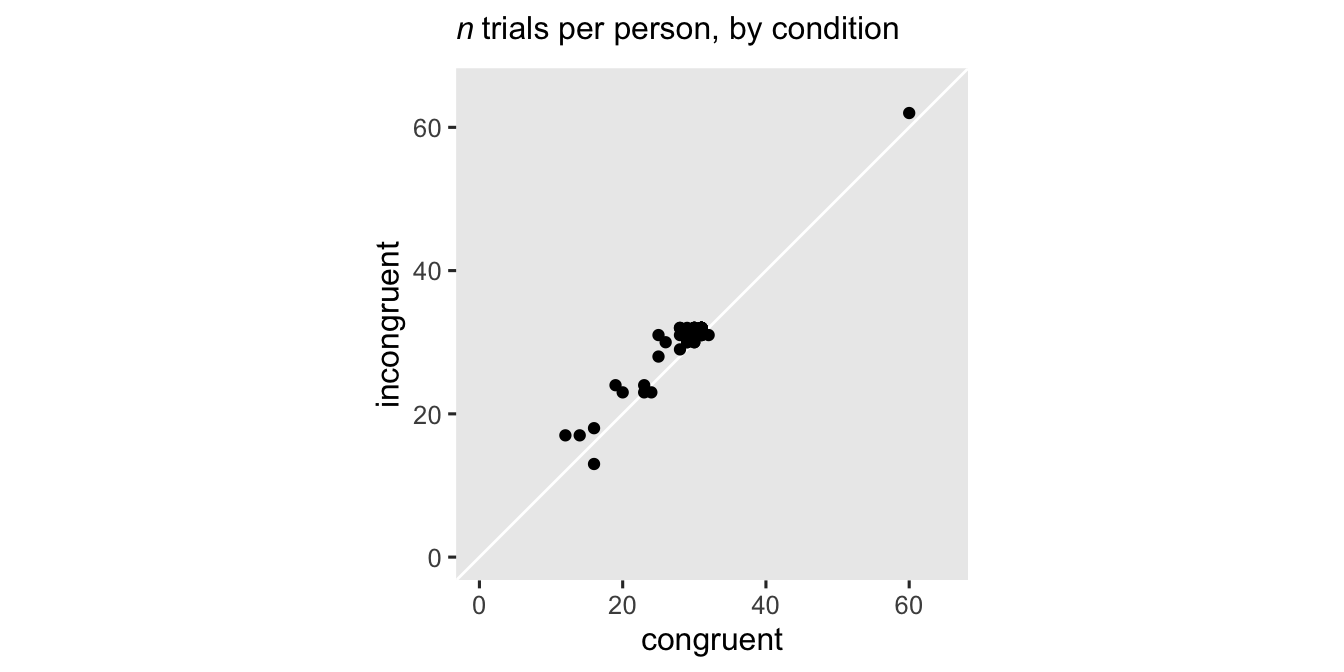
The number of trials differed across participants and conditions, with most ranging between 20 and 40 trials.

stroop_subset |> 
  count(subject, cond) |> 
  pivot_wider(names_from = cond, values_from = n) |> 
  
  ggplot(aes(x = congruent, y = incongruent)) +
  geom_abline(color = "white") +
  geom_point() +
  labs(subtitle = expression(italic(n)~"trials per person, by condition")) +
  coord_equal(xlim = c(0, 65), ylim = c(0, 65))

The levels of cond were randomly assigned to each trial, by participant. To get a sense, here’s a tile plot of the conditions for a random subset of 12 of our focal participants.

set.seed(1)

stroop_subset |> 
  filter(subject %in% sample(random_50_subject, size = 12)) |> 
  mutate(trial = factor(trial)) |> 
  
  ggplot(aes(x = trial, y = subject)) +
  geom_tile(aes(fill = cond), color = "gray92") +
  scale_x_discrete(breaks = NULL) +
  scale_fill_viridis_d(option = "A", end = 0.75)

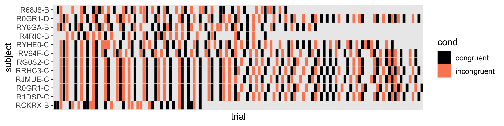
Thus, this is what you might describe as a within-person factorial design. Each person gets many levels of the experimental condition, assigned at random in quick succession. The dependent variable is reaction time in milliseconds (rt). As has long been observed, reaction-time data are often approximately log-normally distributed (e.g., Snodgrass et al., 1967). To give a sense, here’s a plot of rt and log(rt) for the overall subsample.

stroop_subset |> 
  mutate(lrt = log(rt)) |> 
  pivot_longer(cols = c(rt, lrt)) |> 
  mutate(scale = ifelse(name == "lrt", "log(milliseconds)", "milliseconds") |> 
           factor(levels = c("milliseconds", "log(milliseconds)"))) |> 
  
  ggplot(aes(x = value)) +
  geom_histogram(bins = 50) +
  scale_y_continuous(NULL, breaks = NULL) +
  xlab("reaciton time") +
  facet_wrap(~ scale, scales = "free")

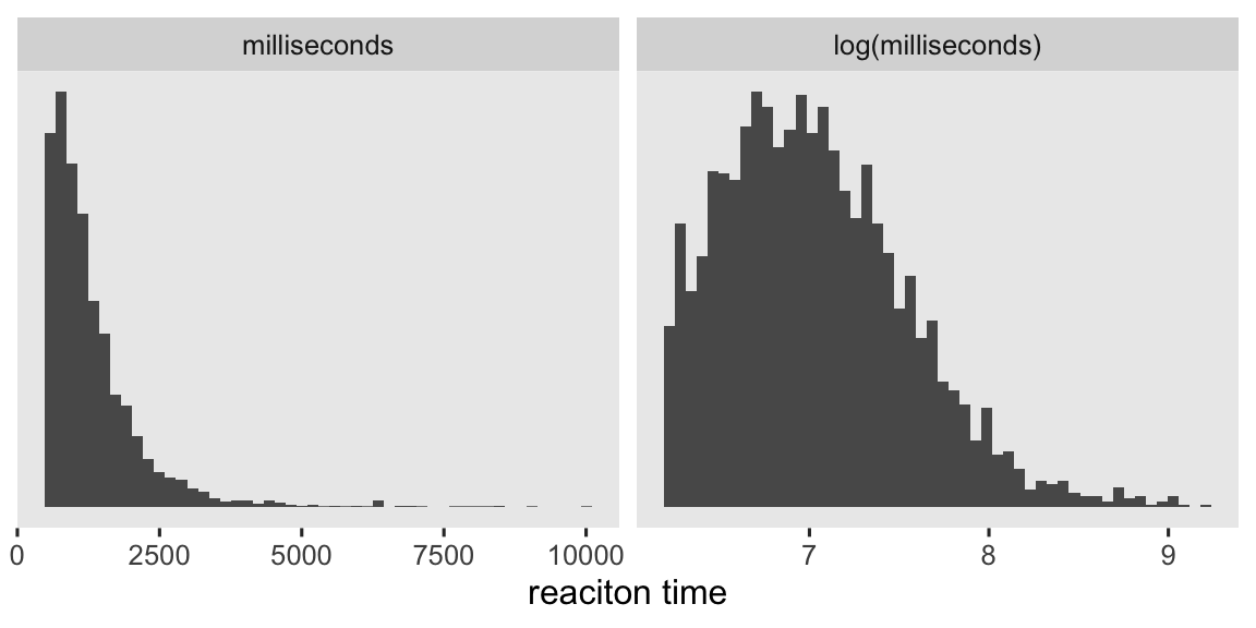
With this data set, we’re playing a little fast and loose calling those data approximately lognormal. But do keep in mind these distributions haven’t yet been conditioned on subject or cond, which can go a long way.

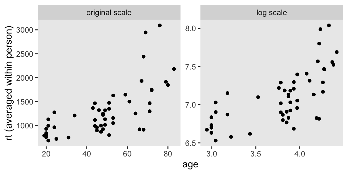
We also have a baseline covariate, age, which you might suspect would have a meaningful association with reaction times. Here’s a scatter plot of age and mean rt.

stroop_subset |> 
  group_by(subject) |> 
  summarise(across(.cols = c(rt, age), .fns = mean)) |> 
  pivot_longer(cols = rt:age, names_to = "variable", values_to = "original") |> 
  mutate(log = log(original)) |> 
  pivot_longer(cols = original:log) |> 
  pivot_wider(names_from = variable, values_from = value) |> 
  mutate(name = factor(name, levels = c("original", "log"), labels = c("original scale", "log scale"))) |> 
  
  ggplot(aes(x = age, y = rt)) +
  geom_point() +
  ylab("rt (averaged within person)") +
  facet_wrap(~ name, scales = "free")

We’ll be using age in our analyses as a background covariate. Here we log transform age (logage), and then mean center that log-transformed version (lac).

stroop_subset <- stroop_subset |> 
  # Log transform `age`
  mutate(logage = log(age)) |> 
  # Mean center `logage`
  mutate(lac = logage - mean(logage))

# How do these three look together?
stroop_subset |> 
  distinct(age, logage, lac) |> 
  arrange(age) |> 
  slice(1, 11:12, 29)

## # A tibble: 4 × 3
##     age logage      lac
##   <int>  <dbl>    <dbl>
## 1    19   2.94 -0.900  
## 2    46   3.83 -0.0159 
## 3    47   3.85  0.00560
## 4    83   4.42  0.574

When the new lac variable is at zero, age is between 46 and 47 years.

Model framework

The primary goal of this post is to walk out causal inference with a multilevel model, which inclines me to stick to a few relatively simple models.⁴ Given the longstanding observation reaction-time data are approximately lognormal, we will simply model log(rt) with the Gaussian likelihood for now. In a later post, however, we will explore how to model rt directly with the lognormal distribution, instead. In this post we will fit two models as frequentists, and then fit two corresponding models as Bayesians.

We start as frequentists.

Frequentist models

Our frequentist multilevel ANOVA will be of the form

$$ \begin{align} \log(\text{rt}_{ij}) & \sim \operatorname{Normal}(\mu_{ij}, \sigma_\epsilon) \\ \mu_{ij} & = \beta_{0i} + \beta_{1i} \text{cond}_{ij} \\ \beta_{0i} & = b_0 + u_{0i} \\ \beta_{1i} & = b_1 + u_{1i} \\ \begin{bmatrix} u_{0i} \\ u_{1i} \end{bmatrix} & \sim \operatorname{Normal} \left ( \mathbf 0, \mathbf \Sigma \right ) \\ \mathbf \Sigma & = \mathbf{SRS} \\ \mathbf S & = \begin{bmatrix} \sigma_{u_0} & \\ 0 & \sigma_{u_1} \end{bmatrix} \\ \mathbf R & = \begin{bmatrix} 1 & \\ \rho & 1 \end{bmatrix}, \end{align} $$

where the dependent variable rt varies across \(i\) participants and \(j\) trials. Its log is modeled as normally distributed, with a conditional mean \(\mu_{ij}\) and residual standard deviation \(\sigma_\epsilon\). The independent variable cond has been defined as a two-level factor for which congruent is the first level, and incongruent is the second. Thus in software, cond will effectively be treated as a dummy variable for which congruent is the reference category and incongruent is the comparison category. Thus the linear model for \(\mu_{ij}\) has an intercept \(\beta_{0i}\) which varies across \(i\) participants, and quantifies their mean values for the congruent condition. The slope \(\beta_{1i}\) is the average difference in the incongruent condition, versus the congruent condition, which also varies across \(i\) participants. In typical multilevel model fashion, we can decompose the intercept \(\beta_{0i}\) into a population mean \(b_0\), and participant-level deviation \(u_{0i}\). In a similar way, we can decompose the slope \(\beta_{1i}\) into a population mean \(b_1\), and participant-level deviation \(u_{1i}\). The two participant-level deviation terms \(u_{0i}\) and \(u_{1i}\) are modeled as bivariate normal with a mean vector of two zeros, and a variance covariance matrix \(\mathbf \Sigma\). Anticipating the needs of our Bayesian brms models below, we can decompose \(\mathbf \Sigma\) into a \(2 \times 2\) matrix for the standard deviations \(\mathbf S\), and a \(2 \times 2\) correlation matrix \(\mathbf R\). On the diagonal of our standard-deviation matrix \(\mathbf S\), we have the standard-deviation terms for \(u_{0i}\) and \(u_{1i}\). On the off-diagonal of our correlation matrix \(\mathbf R\), we have the correlation term for the deviations \(\rho\). The final term \(\sigma_\epsilon\) captures the variation within participants, after accounting for their between-level differences. As is typical, we hold this within-person variance constant across participants.⁵

We can fit the model with restricted maximum likelihood via lmer() like so.

lmer_anova <- lmer(
  data = stroop_subset,
  log(rt) ~ 1 + cond + (1 + cond | subject))

Here’s the model summary.

summary(lmer_anova)

## Linear mixed model fit by REML ['lmerMod']
## Formula: log(rt) ~ 1 + cond + (1 + cond | subject)
##    Data: stroop_subset
## 
## REML criterion at convergence: 2958.4
## 
## Scaled residuals: 
##     Min      1Q  Median      3Q     Max 
## -2.9049 -0.6577 -0.1472  0.4859  6.1498 
## 
## Random effects:
##  Groups   Name            Variance Std.Dev. Corr
##  subject  (Intercept)     0.118881 0.34479      
##           condincongruent 0.003749 0.06123  0.02
##  Residual                 0.149709 0.38692      
## Number of obs: 2921, groups:  subject, 50
## 
## Fixed effects:
##                 Estimate Std. Error t value
## (Intercept)      6.96504    0.04987 139.673
## condincongruent  0.10040    0.01682   5.968
## 
## Correlation of Fixed Effects:
##             (Intr)
## condncngrnt -0.118

Our second model will be a multilevel ANCOVA where we condition on the background variable age, but using the log-transformed and mean-centered version (lac). In our last exploratory figure above, we saw log(age) had a curved relation with the participant-level means for log(rt). To better capture that in the model, we’ll add a quadratic term like so:

$$ \begin{align} \log(\text{rt}_{ij}) & \sim \operatorname{Normal}(\mu_{ij}, \sigma_\epsilon) \\ \mu_{ij} & = \beta_{0i} + \beta_{1i} \text{cond}_{ij} \\ \beta_{0i} & = b_{00} + b_{01} \text{lac}_i + b_{02} \text{lac}_i^2 + u_{0i} \\ \beta_{1i} & = b_1 + u_{1i} \\ \begin{bmatrix} u_{0i} \\ u_{1i} \end{bmatrix} & \sim \operatorname{Normal} \left ( \mathbf 0, \mathbf \Sigma \right ) \\ \mathbf \Sigma & = \mathbf{SRS} \\ \mathbf S & = \begin{bmatrix} \sigma_{u_0} & \\ 0 & \sigma_{u_1} \end{bmatrix} \\ \mathbf R & = \begin{bmatrix} 1 \\ \rho & 1 \end{bmatrix}. \end{align} $$

To accommodate the new terms in the \(\beta_{0i}\), we’ve added a second index for the \(b\)-term subscripts.

Now we fit that mode with lmer().

lmer_ancova <- lmer(
  data = stroop_subset,
  log(rt) ~ 1 + cond + lac + I(lac^2) + (1 + cond | subject))

Here’s the model summary.

summary(lmer_ancova)

## Linear mixed model fit by REML ['lmerMod']
## Formula: log(rt) ~ 1 + cond + lac + I(lac^2) + (1 + cond | subject)
##    Data: stroop_subset
## 
## REML criterion at convergence: 2920.4
## 
## Scaled residuals: 
##     Min      1Q  Median      3Q     Max 
## -2.9226 -0.6595 -0.1446  0.4870  6.1582 
## 
## Random effects:
##  Groups   Name            Variance Std.Dev. Corr 
##  subject  (Intercept)     0.05290  0.23001       
##           condincongruent 0.00368  0.06066  -0.21
##  Residual                 0.14971  0.38693       
## Number of obs: 2921, groups:  subject, 50
## 
## Fixed effects:
##                 Estimate Std. Error t value
## (Intercept)      6.89188    0.04808 143.357
## condincongruent  0.10098    0.01678   6.017
## lac              0.77593    0.10408   7.455
## I(lac^2)         0.54494    0.18608   2.928
## 
## Correlation of Fixed Effects:
##             (Intr) cndncn lac   
## condncngrnt -0.208              
## lac         -0.446  0.000       
## I(lac^2)    -0.700  0.002  0.705

We might compare the population-level experimental contrast parameter \(b_1\), by model.

bind_rows(
  tidy(lmer_anova, conf.int = TRUE, conf.method = "profile"),
  tidy(lmer_ancova, conf.int = TRUE, conf.method = "profile")) |> 
  filter(term == "condincongruent") |> 
  mutate(model = c("anova", "ancova"),
         interval_width = conf.high - conf.low) |> 
  select(model, estimate:conf.high, interval_width)

## # A tibble: 2 × 7
##   model  estimate std.error statistic conf.low conf.high interval_width
##   <chr>     <dbl>     <dbl>     <dbl>    <dbl>     <dbl>          <dbl>
## 1 anova     0.100    0.0168      5.97   0.0669     0.134         0.0667
## 2 ancova    0.101    0.0168      6.02   0.0676     0.134         0.0664

As is often the case, the ANCOVA lent greater precision to \(b_1\) than the ANOVA, though not by much in this case.

Bayesian models

Our first Bayesian model will also be a multilevel ANOVA of the form

$$ \begin{align} \log(\text{rt}_{ij}) & \sim \operatorname{Normal}(\mu_{ij}, \sigma_\epsilon) \\ \mu_{ij} & = \beta_{0i} + \beta_{1i} \text{cond}_{ij} \\ \beta_{0i} & = b_0 + u_{0i} \\ \beta_{1i} & = b_1 + u_{1i} \\ \begin{bmatrix} u_{0i} \\ u_{1i} \end{bmatrix} & \sim \operatorname{Normal} \left ( \mathbf 0, \mathbf \Sigma \right ) \\ \mathbf \Sigma & = \mathbf{SRS} \\ \mathbf S & = \begin{bmatrix} \sigma_{u_0} & \\ 0 & \sigma_{u_1} \end{bmatrix} \\ \mathbf R & = \begin{bmatrix} 1 \\ \rho & 1 \end{bmatrix} \\ b_0 & \sim \operatorname{Normal}(\log 1000, 1) \\ b_1 & \sim \operatorname{Normal}(0, 1) \\ \sigma_{u_0}, \sigma_{u_1}, \sigma_\epsilon & \sim \operatorname{Exponential}(1) \\ \mathbf R & \sim \operatorname{LKJ}(2), \end{align} $$

where the only difference from the frequentist model is we’re now using priors, which are defined in the bottom four rows. All priors are meant to be weakly-regularizing on the scale of the data (the DV of which is on the log scale, keep in mind). We’ll detail each below.

The \(\operatorname{Normal}(\log 1000, 1)\) prior for the population-level intercept \(b_0\) is very weak. We’ve centered the prior on the log of 1000 milliseconds, and 1000 milliseconds is the same as one second. For a given trial on a Stroop task, most folks are going to have reaction times a little above or below a second. In numbers, \(\log 1000 \approx 6.9\). The unit standard deviation on the prior means that about 95% of the prior mass is between 4.9 and 8.9 on the log scale, which is a massive spread. To see the range for yourself, execute exp(log(1000) + c(-2, 2)) in your console. Any experienced Stroop-task researchers should be able to set a much stronger prior than this.

The \(\operatorname{Normal}(0, 1)\) prior for the population-level slope \(b_1\) is also very weak. It would allow for a plus or minus difference of 2 on the log scale for the incongruent condition, relative to the congruent condition. The Stroop effect is very well-established finding in psychology, but as reliable as it is, it’s nowhere near as large as a log difference of 2. Again, an experienced Stroop-task researcher could easily justify a much more specific prior here.

The \(\operatorname{Exponential}(1)\) prior for all three \(\sigma\) parameters is my go-to prior for such parameters any time I’m fitting a model on the log scale. It’s straight out of McElreath ( 2020), and I find it works well for many of the data types I see in psychology.

The \(\operatorname{LKJ}(2)\) prior will gently push the \(\mathbf R\) correlation matrix to have smaller off-diagonal values. For reference, the sole parameter in the LKJ \((\eta)\) ranges from zero to positive infinity. Values of 1 are flat for \(2 \times 2\) matrices such as ours, and small numbers like 2 are very mildly conservative. For more on the LKJ, see Martin ( 2020).

Here’s how to fit the model with brm().

brm_anova <- brm(
  data = stroop_subset,
  family = gaussian,
  bf(log(rt) ~ 1 + cond + (1 + cond | subject),
     center = FALSE),
  prior = prior(normal(log(1000), 1), class = b, coef = Intercept) +
    prior(normal(0, 1), class = b) +
    prior(exponential(1), class = sd) +
    prior(exponential(1), class = sigma) +
    prior(lkj(2), class = cor), 
  cores = 4, seed = 1,
  file = "fits/brm_anova")

Check the summary.

print(brm_anova)

##  Family: gaussian 
##   Links: mu = identity; sigma = identity 
## Formula: log(rt) ~ 1 + cond + (1 + cond | subject) 
##    Data: stroop_subset (Number of observations: 2921) 
##   Draws: 4 chains, each with iter = 2000; warmup = 1000; thin = 1;
##          total post-warmup draws = 4000
## 
## Multilevel Hyperparameters:
## ~subject (Number of levels: 50) 
##                                Estimate Est.Error l-95% CI u-95% CI Rhat
## sd(Intercept)                      0.35      0.04     0.29     0.44 1.01
## sd(condincongruent)                0.05      0.03     0.00     0.10 1.01
## cor(Intercept,condincongruent)     0.05      0.31    -0.56     0.69 1.00
##                                Bulk_ESS Tail_ESS
## sd(Intercept)                       586     1037
## sd(condincongruent)                 482      866
## cor(Intercept,condincongruent)     2759     1758
## 
## Regression Coefficients:
##                 Estimate Est.Error l-95% CI u-95% CI Rhat Bulk_ESS Tail_ESS
## Intercept           6.97      0.05     6.87     7.07 1.01      251      471
## condincongruent     0.10      0.02     0.07     0.13 1.00     4084     3176
## 
## Further Distributional Parameters:
##       Estimate Est.Error l-95% CI u-95% CI Rhat Bulk_ESS Tail_ESS
## sigma     0.39      0.01     0.38     0.40 1.00     4565     3027
## 
## Draws were sampled using sampling(NUTS). For each parameter, Bulk_ESS
## and Tail_ESS are effective sample size measures, and Rhat is the potential
## scale reduction factor on split chains (at convergence, Rhat = 1).

Though not always the case, the parameter summaries for the frequentist and Bayesian ANOVAs are quite similar.

As above in the frequentist models, our second Bayesian model will also be a multilevel ANCOVA where we condition on the background variable lac:

$$ \begin{align} \log(\text{rt}_{ij}) & \sim \operatorname{Normal}(\mu_{ij}, \sigma_\epsilon) \\ \mu_{ij} & = \beta_{0i} + \beta_{1i} \text{cond}_{ij} \\ \beta_{0i} & = b_{00} + b_{01} \text{lac}_i + b_{02} \text{lac}_i^2 + u_{0i} \\ \beta_{1i} & = b_1 + u_{1i} \\ \begin{bmatrix} u_{0i} \\ u_{1i} \end{bmatrix} & \sim \operatorname{Normal} \left ( \mathbf 0, \mathbf \Sigma \right ) \\ \mathbf \Sigma & = \mathbf{SRS} \\ \mathbf S & = \begin{bmatrix} \sigma_{u_0} & \\ 0 & \sigma_{u_1} \end{bmatrix} \\ \mathbf R & = \begin{bmatrix} 1 \\ \rho & 1 \end{bmatrix} \\ b_{00} & \sim \operatorname{Normal}(\log 1000, 1) \\ b_{01}, b_{02}, b_1 & \sim \operatorname{Normal}(0, 1) \\ \sigma_{u_0}, \sigma_{u_1}, \sigma_\epsilon & \sim \operatorname{Exponential}(1) \\ \mathbf R & \sim \operatorname{LKJ}(2). \end{align} $$

For the priors, \(\operatorname{Normal}(0, 1)\) should be pretty gentle for both \(b_{01}\) and \(b_{02}\). Because we have mean-centered lac, I feel comfortable retaining the \(\operatorname{Normal}(\log 1000, 1)\) prior for \(b_{00}\).

We can fit the multilevel ANCOVA with brm() like so.

brm_ancova <- brm(
  data = stroop_subset,
  family = gaussian,
  bf(log(rt) ~ 1 + cond + lac + I(lac^2) + (1 + cond | subject),
     center = FALSE),
  prior = prior(normal(log(1000), 1), class = b, coef = Intercept) +
    prior(normal(0, 1), class = b) +
    prior(exponential(1), class = sd) +
    prior(exponential(1), class = sigma) +
    prior(lkj(2), class = cor),
  cores = 4, seed = 1,
  file = "fits/brm_ancova")

Check the parameter summary.

print(brm_ancova)

##  Family: gaussian 
##   Links: mu = identity; sigma = identity 
## Formula: log(rt) ~ 1 + cond + lac + I(lac^2) + (1 + cond | subject) 
##    Data: stroop_subset (Number of observations: 2921) 
##   Draws: 4 chains, each with iter = 2000; warmup = 1000; thin = 1;
##          total post-warmup draws = 4000
## 
## Multilevel Hyperparameters:
## ~subject (Number of levels: 50) 
##                                Estimate Est.Error l-95% CI u-95% CI Rhat
## sd(Intercept)                      0.24      0.03     0.19     0.30 1.01
## sd(condincongruent)                0.05      0.03     0.00     0.10 1.00
## cor(Intercept,condincongruent)    -0.13      0.32    -0.71     0.57 1.00
##                                Bulk_ESS Tail_ESS
## sd(Intercept)                       718     1204
## sd(condincongruent)                 542     1018
## cor(Intercept,condincongruent)     2178     1746
## 
## Regression Coefficients:
##                 Estimate Est.Error l-95% CI u-95% CI Rhat Bulk_ESS Tail_ESS
## Intercept           6.89      0.05     6.80     6.99 1.00      488      821
## condincongruent     0.10      0.02     0.07     0.13 1.00     2784     2357
## lac                 0.76      0.10     0.56     0.96 1.00      555      856
## IlacE2              0.53      0.18     0.18     0.87 1.00      585     1032
## 
## Further Distributional Parameters:
##       Estimate Est.Error l-95% CI u-95% CI Rhat Bulk_ESS Tail_ESS
## sigma     0.39      0.01     0.38     0.40 1.00     3972     2701
## 
## Draws were sampled using sampling(NUTS). For each parameter, Bulk_ESS
## and Tail_ESS are effective sample size measures, and Rhat is the potential
## scale reduction factor on split chains (at convergence, Rhat = 1).

At first glance, the \(b_{01}\) and \(b_{02}\) posteriors might seem strong. Keep in mind the lac variable only ranges from -0.900 (age == 19) to 0.574 (age == 83), so a one-unit increase in lac is a massive increase on the age scale.⁶ Take together, the \(b_{01}\) and \(b_{02}\) posteriors indicate that older participants tended to have longer reaction times, and this trend increased on the right end of the age distribution.

We might make a couple gross pp_check() plots to get a sense of the quality of our models.

set.seed(1)
p1 <- pp_check(brm_anova, ndraws = 50) + 
  coord_cartesian(xlim = c(5, 9), ylim = c(0, 0.8)) +
  labs(subtitle = "ANOVA")
p2 <- pp_check(brm_ancova, ndraws = 50) + 
  coord_cartesian(xlim = c(5, 9), ylim = c(0, 0.8)) +
  labs(subtitle = "ANCOVA")

p1 / p2

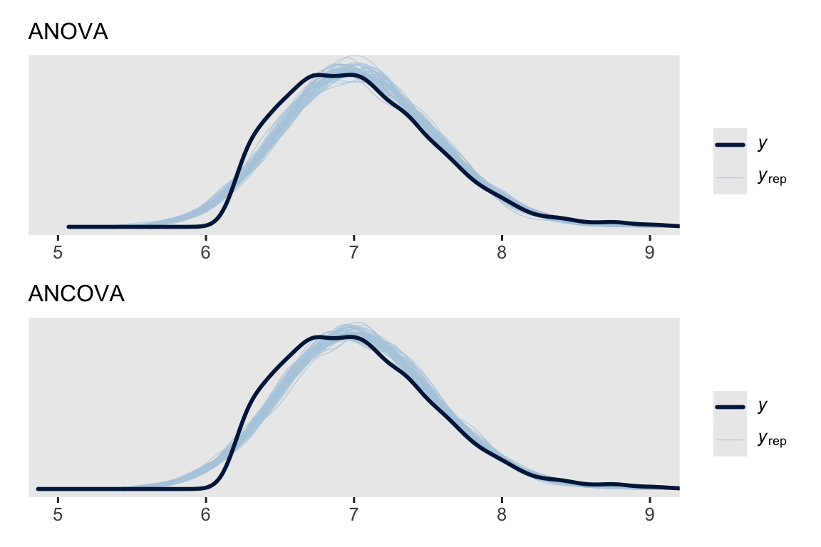
Overall, they’re not great. But they do at least capture the conditional means.⁷

set.seed(1)
p3 <- pp_check(brm_anova, type = "stat_grouped", group = "cond", ndraws = 2000) + 
  coord_cartesian(xlim = c(6.94, 7.13)) +
  labs(subtitle = "ANOVA")
p4 <- pp_check(brm_ancova, type = "stat_grouped", group = "cond", ndraws = 2000) + 
  coord_cartesian(xlim = c(6.94, 7.13)) +
  labs(subtitle = "ANCOVA")

p3 / p4

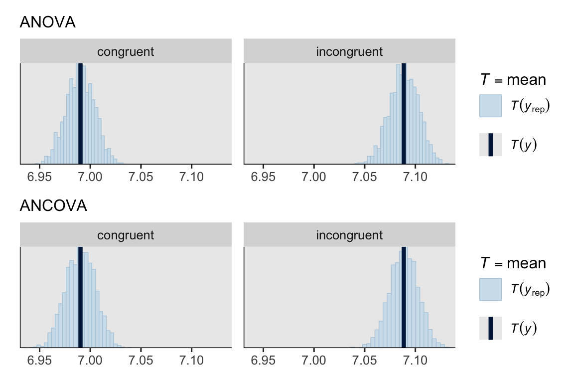
Given the strength of our \(b_{01}\) and \(b_{02}\) posteriors, we might expect greater precision for our population-level experimental contrast parameter \(b_1\).

bind_rows(
  fixef(brm_anova)["condincongruent", ],
  fixef(brm_ancova)["condincongruent", ]) |> 
  mutate(model = c("anova", "ancova"),
         interval_width = Q97.5 - Q2.5) |> 
  select(model, everything())

## # A tibble: 2 × 6
##   model  Estimate Est.Error   Q2.5 Q97.5 interval_width
##   <chr>     <dbl>     <dbl>  <dbl> <dbl>          <dbl>
## 1 anova     0.100    0.0165 0.0682 0.133         0.0653
## 2 ancova    0.101    0.0166 0.0675 0.134         0.0660

In this case, the contrast is mixed. With respect for the the posterior \(\textit{SD}\), the value is smaller for the ANOVA. But the 95% interval is narrower for the ANCOVA. We’ll have to see what happens for the causal estimands, below.

Causal inference with multilevel models

When we measure the dependent variable at a single time point, we can define the causal effect \(\tau\) of one condition versus another for the \(i\)th person as

$$ \tau_i = y_i^1 - y_i^0, $$

where \(y_i^0\) is the \(i\)th person’s outcome in one condition,⁸ and where \(y_i^1\) is the \(i\)th person’s outcome in other condition.⁹ Within-person factorial experiments add a temporal element where the DV is measured across many trials, where the level of the independent variable is varied (often at random, as in these data). Thus in a technical sense, reaction-time data like these are longitudinal, though you might describe them as intensively longitudinal.¹⁰ Therefore we might need to expand our notation to capture the response across \(j\) time points (trials), and define the \(i\)th person’s causal effect at a given time point as

$$ \tau_{ij} = y_{ij}^1 - y_{ij}^0. $$

We often express causal effects in aggregates, and within-person designs allow for several options. For example, if we wanted to average across all \(j\) trials within each \(i\) persons, we could compute a person-specific average treatment effect (ATE):

$$ \tau_{\text{ATE}_i} = \mathbb E (y_j^1 - y_j^0)_i. $$

If we were instead interested in averaging across \(i\) persons, we could compute a trail-specific ATE:

$$ \tau_{\text{ATE}_j} = \mathbb E (y_i^1 - y_i^0)_j. $$

Often times researchers simply want a causal effect averaged across trials and persons:

$$ \tau_\text{ATE} = \mathbb E (y_{ij}^1 - y_{ij}^0). $$

Yet keep in mind that even though each participant receives multiple trials under both levels of the independent variable, \(\tau_{ij}\) can never be directly computed from the data alone because for any given trial \(j\), the \(i\)th participant is only under one of the levels of the independent variable. Thus Holland’s ( 1986) fundamental problem of causal inference still holds even when we have many observations within each person: We are always missing at least half of the data. This would also hold true for other within-person designs, such as the crossover trials used in medicine and exercise science (see Senn, 2002), or the reversal designs used in behavior analysis and education research (see Cooper et al., 2019).

However, as we have seen on previous posts, we can use g-computation ( Robins, 1986) to compute estimates for \(y_{ij}^1\) and \(y_{ij}^0\) from the model, and then average over those estimates to ATE. We can compute these estimates from an unconditional model, such as a multilevel ANOVA, or a conditional model, such as a multilevel ANCOVA.

As we saw in the first blog series, sometimes the ATE is directly estimated from one of the parameters in the model (often \(\beta_1\) in a single-level Gaussian ANOVA or ANCOVA), but sometimes the ATE is only a product of the entire model realized through g-computation (as is often the case when using a non-identity link function). It is my observation that for multilevel models, the ATE requires g-computation, with caveats we’ll highlight below.¹¹

For more theory on causal inference with multilevel models in other research design contexts, see Hill ( 2013), Feller & Gelman ( 2015), and Raudenbush & Schwartz ( 2020).

Frequentist g-computation

Frequentist ANOVA and the ATE

If we took the generic \(\tau_\text{ATE}\) as our focal estimand, we can compute the point estimate by hand following the same basic steps for with a single-level GLM. The first step is to make a predictor grid of all the model inputs. For that grid, we start with the observed levels of subject. Though not technically necessary at this point, it can help clarify the steps by retaining the trial indices. We then double the length of the data set such that the first version has one level of the IV for all cases (cond == "congruent"), and the other level of the IV for the duplicate cases (cond == "incongruent"). We save the predictor grid as nd, my preferred shorthand for newdata.

nd <- stroop_subset |> 
  # Subset the necessary columns
  select(subject, trial) |> 
  # Expand the data set by the two levels of the IV
  expand_grid(cond = levels(stroop_subset$cond) |> 
                factor(levels = levels(stroop_subset$cond)))

# What?
glimpse(nd)

## Rows: 5,842
## Columns: 3
## $ subject <fct> R08T1-C, R08T1-C, R08T1-C, R08T1-C, R08T1-C, R08T1-C, R08T1-C,…
## $ trial   <int> 3, 3, 4, 4, 5, 5, 8, 8, 10, 10, 12, 12, 14, 14, 16, 16, 19, 19…
## $ cond    <fct> congruent, incongruent, congruent, incongruent, congruent, inc…

Here’s the structure of the output of predict() when you request se = TRUE.

predict(lmer_anova, newdata = nd, se = TRUE) |> 
  str()

## List of 2
##  $ fit   : Named num [1:5842] 7.11 7.22 7.11 7.22 7.11 ...
##   ..- attr(*, "names")= chr [1:5842] "1" "2" "3" "4" ...
##  $ se.fit: Named num [1:5842] 0.055 0.0552 0.055 0.0552 0.055 ...
##   ..- attr(*, "names")= chr [1:5842] "1" "2" "3" "4" ...

In late 2023 lme4 began offering an se.fit = TRUE method for the predict() function. If you execute ?predict.merMod for the documentation, you will find this method is currently considered “experimental”. There is no current direct method to request 95% CIs, but you can compute Wald intervals by hand. Exciting as it is, the se.fit = TRUE method won’t actually serve us well here because we’re interested in averaging across the trial-level estimates with subjects, and we’ll be interested in computing within-subject contrasts from them as well.

Before we move on, an important thing to notice is that for a simple multilevel ANOVA like this, all counterfactual predictions will be identical across all levels of trial per subject, within each level of the IV. This might be easier to see if we slice() to show the last three trials for the first subject, and the first three trials for the second.

nd |> 
  mutate(y_hat = predict(lmer_anova, newdata = nd)) |> 
  pivot_wider(names_from = cond, values_from = y_hat) |> 
  slice(61:66)

## # A tibble: 6 × 4
##   subject trial congruent incongruent
##   <fct>   <int>     <dbl>       <dbl>
## 1 R08T1-C   120      7.11        7.22
## 2 R08T1-C   123      7.11        7.22
## 3 R08T1-C   125      7.11        7.22
## 4 R0GR1-C     3      7.14        7.21
## 5 R0GR1-C     4      7.14        7.21
## 6 R0GR1-C     5      7.14        7.21

See? All the expected values in congruent are all the same for each level of subject, as are the all the expected values for incongruent. Because the simple multilevel ANOVA has no way to capture systemic differences across trials within a subject, this holds for all trials within all levels of subject. In a later post, we’ll see how we might model systemic within-subject differences.

As with single-level GLMs, we can also compute counterfactual estimates with predictions() from marginaleffects. Here’s the default output.

lmer_anova_predictions_ij <- predictions(lmer_anova, newdata = nd)

## Warning: For this model type, `marginaleffects` only takes into account the
## uncertainty in fixed-effect parameters. This is often appropriate when
## `re.form=NA`, but may be surprising to users who set `re.form=NULL` (default)
## or to some other value. Call `options(marginaleffects_safe = FALSE)` to silence
## this warning.

head(lmer_anova_predictions_ij)

## 
##  Estimate Std. Error   z Pr(>|z|)   S 2.5 % 97.5 %
##      7.11     0.0499 143   <0.001 Inf  7.01   7.20
##      7.22     0.0507 142   <0.001 Inf  7.12   7.32
##      7.11     0.0499 143   <0.001 Inf  7.01   7.20
##      7.22     0.0507 142   <0.001 Inf  7.12   7.32
##      7.11     0.0499 143   <0.001 Inf  7.01   7.20
##      7.22     0.0507 142   <0.001 Inf  7.12   7.32
## 
## Type: response

Notice the warning message, which begins: “For this model type, marginaleffects only takes into account the uncertainty in fixed-effect parameters.” Although we do have correct point estimates in the Estimate column, we should not trust the standard errors or any of the products of the standard errors, such as the \(p\)-value and 95% CI. Those standard errors are based only on the fixed effects, which ignore the uncertainty in the random portion of the model. This is because, for frequentist models, marginaleffects only uses the output of the vcov() function as input for its own implementation of the delta method. The vcov() function will return the variance/covariance matrix for the fixed effects (what we called \(b\) coefficients in our equations, above), but it does not include uncertainty information for the multilevel deviation parameters (often called random effects, and what we called \(u\) parameter, above). However, one can compute frequentist 95% CIs with bootstrapping, which we’ll show in a moment. But first, we can use the by argument in the avg_predictions() function to compute the average estimates, within each level cond, within each level of subject. These are what we might denote \(\mathbb E (y_j^0)_i\) and \(\mathbb E (y_j^1)_i\).

lmer_anova_predictions_i <- avg_predictions(
  lmer_anova, 
  newdata = nd, 
  by = c("subject", "cond"))

head(lmer_anova_predictions_i)

## 
##  subject        cond Estimate Std. Error   z Pr(>|z|)   S 2.5 % 97.5 %
##  RCKRX-B congruent       6.73     0.0499 135   <0.001 Inf  6.63   6.82
##  RCKRX-B incongruent     6.82     0.0507 134   <0.001 Inf  6.72   6.91
##  RRVBZ-C congruent       6.63     0.0499 133   <0.001 Inf  6.53   6.73
##  RRVBZ-C incongruent     6.68     0.0507 132   <0.001 Inf  6.58   6.78
##  R8EZH-D congruent       7.39     0.0499 148   <0.001 Inf  7.29   7.49
##  R8EZH-D incongruent     7.52     0.0507 148   <0.001 Inf  7.42   7.62
## 
## Type: response

I’ve suppressed the warning message here, but you’ll still get one. You should not trust those standard errors, even though the point estimates are fine. To express uncertainty with bootstrap 95% CIs, we use the inferences() function from marginaleffects (execute ?inferences for the documentation). Here we use the rsample method, and compute the intervals based on 1000 bootstraped samples. This operation takes about a minute on my laptop, so make sure to save the results as an object when you do something like this on your own computer.¹²

lmer_anova_predictions_i_boot <- inferences(
  lmer_anova_predictions_i, 
  method = "rsample", 
  R = 1000)

head(lmer_anova_predictions_i_boot)

## 
##  subject        cond Estimate 2.5 % 97.5 %
##  RCKRX-B congruent       6.73  6.56   6.96
##  RCKRX-B incongruent     6.82  6.67   6.96
##  RRVBZ-C congruent       6.63  6.59   6.71
##  RRVBZ-C incongruent     6.68  6.56   6.75
##  R8EZH-D congruent       7.39  7.26   7.49
##  R8EZH-D incongruent     7.52  7.41   7.65
## 
## Type: response

The object now contains two new columns for the 95% bootstrap CIs.

We can follow similar steps to compute the average within-subject contrasts with avg_comparisons(), what we might denote \(\tau_{\text{ATE}_i}\).

lmer_anova_comparisons_i <- avg_comparisons(
  lmer_anova, newdata = nd, variables = "cond", by = "subject")
lmer_anova_comparisons_i_boot <- inferences(
  lmer_anova_comparisons_i, method = "rsample", R = 1000)
head(lmer_anova_comparisons_i_boot)

## 
##  subject Estimate   2.5 % 97.5 %
##  RCKRX-B   0.0889 -0.0714 0.1931
##  RRVBZ-C   0.0480 -0.0882 0.0802
##  R8EZH-D   0.1305  0.0317 0.2788
##  R1DSP-C   0.0764 -0.0202 0.1199
##  RAUUJ-C   0.1033 -0.0405 0.2458
##  RGA7X-D   0.0857 -0.0343 0.1502
## 
## Term: cond
## Type: response
## Comparison: incongruent - congruent

Though not strictly necessary, we’ll also compute a rank based on each \(\mathbb E (y_j^0)_i\) estimate to aid with the plots.

# Compute the ranks and save as a simple data frame
ranks <- lmer_anova_predictions_i |> 
  data.frame() |> 
  filter(cond == "congruent") |> 
  mutate(rank = rank(estimate)) |> 
  select(subject, rank)

# What?
glimpse(ranks)

## Rows: 50
## Columns: 2
## $ subject <fct> RCKRX-B, RRVBZ-C, R8EZH-D, R1DSP-C, RAUUJ-C, RGA7X-D, R3QC8-C,…
## $ rank    <dbl> 14, 8, 45, 25, 34, 42, 41, 49, 2, 37, 47, 15, 17, 27, 33, 23, …

Now we plot.

# Counterfactual prediction means
p1 <- lmer_anova_predictions_i_boot |> 
  data.frame() |> 
  mutate(y = ifelse(cond == "congruent", "E(widehat(italic(y[j])^0))[italic(i)]", "E(widehat(italic(y[j])^1))[italic(i)]")) |> 
  left_join(ranks, by = "subject") |> 
  
  ggplot(aes(x = estimate, y = reorder(subject, rank), color = y)) +
  geom_interval(aes(xmin = conf.low, xmax = conf.high),
                position = position_dodge(width = -0.3),
                size = 1/5) +
  geom_point(aes(shape = y),
             size = 2) +
  scale_y_discrete(breaks = NULL) +
  scale_color_viridis_d(NULL, option = "A", begin = 0.3, end = 0.6,
                        labels = scales::parse_format()) +
  scale_shape_manual(NULL, values = c(20, 18),
                     labels = scales::parse_format()) +
  guides(color = guide_legend(position = "inside"),
         shape = guide_legend(position = "inside")) +
  labs(x = "log(rt)",
       y = "subject (ranked)",
       subtitle = "Counterfactual prediction means") +
  coord_cartesian(xlim = c(6.3, 8.2)) +
  theme(legend.background = element_blank(),
        legend.position.inside = c(0.85, 0.75))

# Experimental effects
p2 <- lmer_anova_comparisons_i_boot |>  
  data.frame() |> 
  left_join(ranks, by = "subject") |>
  
  ggplot(aes(x = estimate, y = reorder(subject, rank))) +
  geom_vline(xintercept = 0, color = "white") +
  geom_interval(aes(xmin = conf.low, xmax = conf.high),
                size = 1/5) +
  geom_point() +
  scale_y_discrete(breaks = NULL) +
  labs(x = expression(hat(tau)[italic(i)]~("i.e., "*E(widehat(italic(y[j])^1-italic(y[j])^0))[italic(i)])),
       y = NULL,
       subtitle = "Experimental effects") +
  coord_cartesian(xlim = c(-0.95, 0.95)) 

# Combine, entitle, and display
p1 + p2 + plot_annotation(title = "Person-level estimates based on the frequentist multilevel ANOVA")

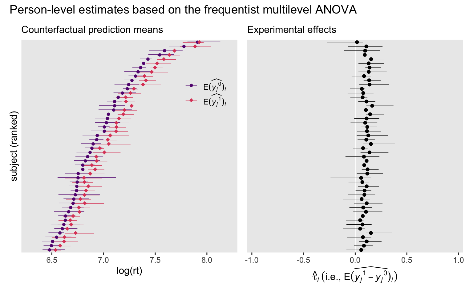
See those horizontal lines? Those are those 95% bootstrap CIs we’ve been working so hard for. Unlike with the single-level GLM ANOVAs we have seen before ( here), even the simple multilevel ANOVA allows the counterfactual estimates and causal effects to vary across persons. This is because the multilevel model groups the trial-level observations within subject for both intercepts and slopes.¹³

Now let’s see what happens if we average across all those \(\tau_{ij}\) estimates.

lmer_anova_comparisons <- avg_comparisons(lmer_anova)
lmer_anova_comparisons_boot <- inferences(
  lmer_anova_comparisons, method = "rsample", R = 1000)
print(lmer_anova_comparisons_boot)

## 
##  Estimate  2.5 % 97.5 %
##     0.101 0.0769  0.129
## 
## Term: cond
## Type: response
## Comparison: incongruent - congruent

This is our overall ATE, with uncertainty expressed with 95% bootstrapped CIs. Note how it’s similar, but not the same as, the estimate for \(b_1\). The 95% CI for that parameter is wider.

tidy(lmer_anova, conf.int = TRUE, conf.method = "profile") |> 
  filter(term == "condincongruent") |> 
  select(estimate, conf.low:conf.high)

## # A tibble: 1 × 3
##   estimate conf.low conf.high
##      <dbl>    <dbl>     <dbl>
## 1    0.100   0.0669     0.134

The point estimate for \(b_1\) is very similar to the point estimate for our ATE, but they’re not identical. This is important to get. The population-level slope \(b_1\) from our multilevel ANOVA is not the same as the ATE. To the best of my knowledge, the two do approximate one another. But whereas our causal estimand is the ATE, \(b_1\) is just a part of the model we use to compute the ATE. That is, in the multilevel ANOVA

$$\tau_\text{ATE} \neq b_1.$$

Frequentist ANCOVA and the ATE

To compute our estimands from our frequentist ANCOVA, we’ll want to add the age variables to the nd predictor grid.

nd <- nd |> 
  left_join(stroop_subset |> 
              distinct(subject, age, lac),
            by = join_by(subject))

# What?
glimpse(nd)

## Rows: 5,842
## Columns: 5
## $ subject <fct> R08T1-C, R08T1-C, R08T1-C, R08T1-C, R08T1-C, R08T1-C, R08T1-C,…
## $ trial   <int> 3, 3, 4, 4, 5, 5, 8, 8, 10, 10, 12, 12, 14, 14, 16, 16, 19, 19…
## $ cond    <fct> congruent, incongruent, congruent, incongruent, congruent, inc…
## $ age     <int> 51, 51, 51, 51, 51, 51, 51, 51, 51, 51, 51, 51, 51, 51, 51, 51…
## $ lac     <dbl> 0.08727658, 0.08727658, 0.08727658, 0.08727658, 0.08727658, 0.…

The remaining steps are much the same. We can compute point estimates for predictions and contrasts with functions like predictions(), comparisons(), avg_predictions(), and avg_comparisons(). But for measures of uncertainty, we bootstrap with inferences().

First, we compute the estimates for \(\mathbb E (y_j^0)_i\) and \(\mathbb E (y_j^1)_i\).

lmer_ancova_predictions_i <- avg_predictions(
  lmer_ancova, newdata = nd, by = c("subject", "cond"))
lmer_ancova_predictions_i_boot <- inferences(
  lmer_ancova_predictions_i, method = "rsample", R = 1000)
head(lmer_ancova_predictions_i_boot)

## 
##  subject        cond Estimate 2.5 % 97.5 %
##  RCKRX-B congruent       6.71  6.55   6.94
##  RCKRX-B incongruent     6.80  6.66   6.93
##  RRVBZ-C congruent       6.63  6.60   6.72
##  RRVBZ-C incongruent     6.69  6.57   6.76
##  R8EZH-D congruent       7.40  7.27   7.50
##  R8EZH-D incongruent     7.53  7.43   7.65
## 
## Type: response

Next we compute and save \(\tau_{j}\) estimates from the frequentist multilevel ANCOVA.

lmer_ancova_comparisons_i <- avg_comparisons(
  lmer_ancova, newdata = nd, variables = "cond", by = "subject")
lmer_ancova_comparisons_i_boot <- inferences(
  lmer_ancova_comparisons_i, method = "rsample", R = 1000)
head(lmer_ancova_comparisons_i_boot)

## 
##  subject Estimate   2.5 % 97.5 %
##  RCKRX-B   0.0913 -0.0875 0.2102
##  RRVBZ-C   0.0597 -0.0847 0.0877
##  R8EZH-D   0.1253  0.0361 0.2823
##  R1DSP-C   0.0801 -0.0185 0.1197
##  RAUUJ-C   0.0998 -0.0542 0.2550
##  RGA7X-D   0.0785 -0.0342 0.1487
## 
## Term: cond
## Type: response
## Comparison: incongruent - congruent

We can plot like before.

# Counterfactual prediction means
p3 <- lmer_ancova_predictions_i_boot |> 
  data.frame() |> 
  mutate(y = ifelse(cond == "congruent", "E(widehat(italic(y[j])^0))[italic(i)]", "E(widehat(italic(y[j])^1))[italic(i)]")) |> 
  left_join(ranks, by = "subject") |> 
  
  ggplot(aes(x = estimate, y = reorder(subject, rank), color = y)) +
  geom_interval(aes(xmin = conf.low, xmax = conf.high),
                position = position_dodge(width = -0.3),
                size = 1/5) +
  geom_point(aes(shape = y),
             size = 2) +
  scale_y_discrete(breaks = NULL) +
  scale_color_viridis_d(NULL, option = "A", begin = 0.3, end = 0.6,
                        labels = scales::parse_format()) +
  scale_shape_manual(NULL, values = c(20, 18),
                     labels = scales::parse_format()) +
  guides(color = guide_legend(position = "inside"),
         shape = guide_legend(position = "inside")) +
  labs(x = "log(rt)",
       y = "subject (ranked)",
       subtitle = "Counterfactual prediction means") +
  coord_cartesian(xlim = c(6.3, 8.2)) +
  theme(legend.background = element_blank(),
        legend.position.inside = c(0.85, 0.75))

# Experimental effects
p4 <- lmer_ancova_comparisons_i_boot |>  
  data.frame() |> 
  left_join(ranks, by = "subject") |>
  
  ggplot(aes(x = estimate, y = reorder(subject, rank))) +
  geom_vline(xintercept = 0, color = "white") +
  geom_interval(aes(xmin = conf.low, xmax = conf.high),
                size = 1/5) +
  geom_point() +
  scale_y_discrete(breaks = NULL) +
  labs(x = expression(hat(tau)[italic(i)]~("i.e., "*E(widehat(italic(y[j])^1-italic(y[j])^0))[italic(i)])),
       y = NULL,
       subtitle = "Experimental effects") +
  coord_cartesian(xlim = c(-0.95, 0.95)) 

# Combine, entitle, and display
p3 + p4 + plot_annotation(title = "Person-level estimates based on the frequentist multilevel ANCOVA")

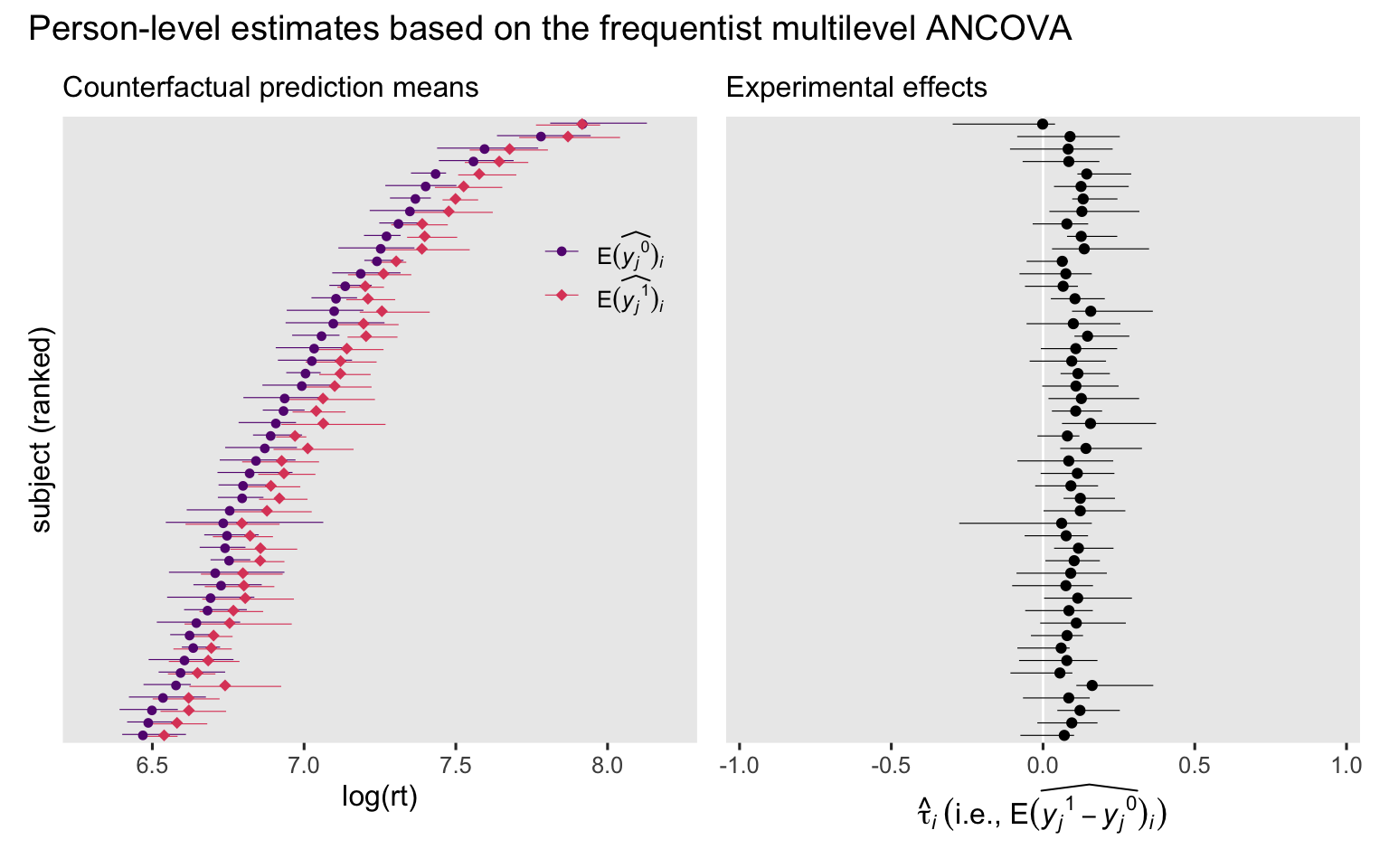
In this case, the results are pretty close to what we got from the ANOVA. Conditioning on age helped a bit, but not a lot compared to what we already got from conditioning on subject. We can get a sense of this with a quick AIC comparison.

AIC(lmer_anova, lmer_ancova)

##             df      AIC
## lmer_anova   6 2970.383
## lmer_ancova  8 2936.387

The ANCOVA captured more information in the data, but not dramatically so.

Now we compute the estimate for the ATE.

lmer_ancova_comparisons <- avg_comparisons(
  lmer_ancova, variables = "cond")
lmer_ancova_comparisons_boot <- inferences(
  lmer_ancova_comparisons, method = "rsample", R = 1000)
print(lmer_ancova_comparisons_boot)

## 
##  Estimate  2.5 % 97.5 %
##     0.101 0.0747  0.129
## 
## Term: cond
## Type: response
## Comparison: incongruent - congruent

To summarize, we might compare the \(b_1\) and \(\tau_\text{ATE}\) estimates from the frequentist ANOVA and ANCOVA all in one coefficient plot.

# Compute
frequentist_ates <- bind_rows(
  lmer_anova_comparisons_boot,
  lmer_ancova_comparisons_boot) |> 
  data.frame() |> 
  mutate(model = c("ANOVA", "ANCOVA"),
         statistic = "ATE") |> 
  select(model, statistic, estimate, contains("conf."))

frequentist_b1s <- bind_rows(
  tidy(lmer_anova, conf.int = TRUE, conf.method = "profile"),
  tidy(lmer_ancova, conf.int = TRUE, conf.method = "profile")) |> 
  filter(term == "condincongruent") |> 
  mutate(model = c("ANOVA", "ANCOVA"),
         statistic = "italic(b)[1]") |> 
  select(model, statistic, estimate, contains("conf."))

# Combine
bind_rows(
  frequentist_ates,
  frequentist_b1s) |> 
  mutate(model = fct_rev(model)) |> 
  
  # Plot
  ggplot(aes(x = estimate, xmin = conf.low, xmax = conf.high, y = model, color = statistic)) +
  geom_vline(xintercept = 0, color = "white") +
  geom_pointinterval(position = position_dodge(width = -0.5), size = 1.5) +
  scale_color_viridis_d(NULL, option = "C", begin = 0.25, end = 0.5, labels = scales::parse_format()) +
  labs(x = "parameter space",
       y = NULL)

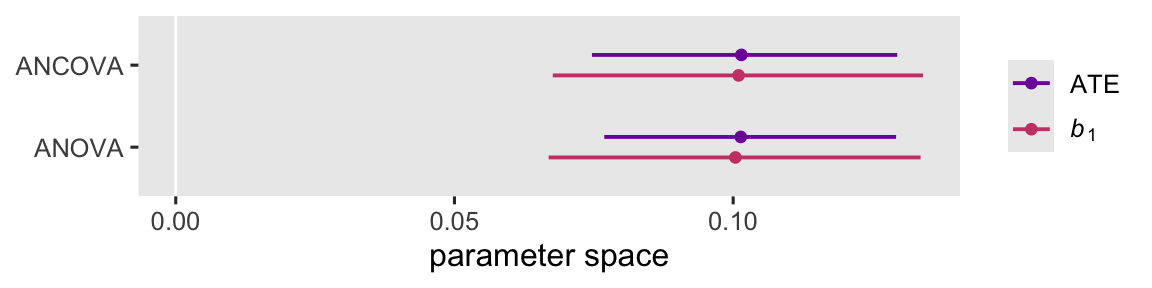
Within and across models, \(b_1\) and \(\tau_\text{ATE}\) approximate one another. However, across both models \(\tau_\text{ATE}\) is more precise than \(b_1\). In this particular case, the multilevel ANCOVA isn’t an improvement over the multilevel ANCOVA with respect to precision.¹⁴ This difference between \(b_1\) and \(\tau_\text{ATE}\), however, is important from a study-design perspective. If it is generally the case that the ATE computed via g-computation is more precise than the population parameter \(b_1\), then that means for a given sample the ATE will have more statistical power, which wise researchers can account for when the plan for their studies with power analyses.

Bayesian g-computation

Bayesian ANOVA and the ATE

There are numerous ways to compute expected values for our predictor grid, and we’ll start with the add_epred_draws() method.

brm_anova_epred_ij <- nd |> 
  add_epred_draws(brm_anova)

# What?
glimpse(brm_anova_epred_ij)

## Rows: 23,368,000
## Columns: 10
## Groups: subject, trial, cond, age, lac, .row [5,842]
## $ subject    <fct> R08T1-C, R08T1-C, R08T1-C, R08T1-C, R08T1-C, R08T1-C, R08T1…
## $ trial      <int> 3, 3, 3, 3, 3, 3, 3, 3, 3, 3, 3, 3, 3, 3, 3, 3, 3, 3, 3, 3,…
## $ cond       <fct> congruent, congruent, congruent, congruent, congruent, cong…
## $ age        <int> 51, 51, 51, 51, 51, 51, 51, 51, 51, 51, 51, 51, 51, 51, 51,…
## $ lac        <dbl> 0.08727658, 0.08727658, 0.08727658, 0.08727658, 0.08727658,…
## $ .row       <int> 1, 1, 1, 1, 1, 1, 1, 1, 1, 1, 1, 1, 1, 1, 1, 1, 1, 1, 1, 1,…
## $ .chain     <int> NA, NA, NA, NA, NA, NA, NA, NA, NA, NA, NA, NA, NA, NA, NA,…
## $ .iteration <int> NA, NA, NA, NA, NA, NA, NA, NA, NA, NA, NA, NA, NA, NA, NA,…
## $ .draw      <int> 1, 2, 3, 4, 5, 6, 7, 8, 9, 10, 11, 12, 13, 14, 15, 16, 17, …
## $ .epred     <dbl> 7.053134, 7.050039, 7.176576, 7.046414, 7.134323, 7.187468,…

Next we pivot to the wide format with respect to the two levels of cond, and then compute \(\tau_{ij}\).

brm_anova_epred_ij <- brm_anova_epred_ij |> 
  ungroup() |> 
  select(subject:cond, .draw, .epred) |> 
  pivot_wider(names_from = cond, values_from = .epred) |> 
  mutate(tau_ij = incongruent - congruent)

# What?
glimpse(brm_anova_epred_ij)

## Rows: 11,684,000
## Columns: 6
## $ subject     <fct> R08T1-C, R08T1-C, R08T1-C, R08T1-C, R08T1-C, R08T1-C, R08T…
## $ trial       <int> 3, 3, 3, 3, 3, 3, 3, 3, 3, 3, 3, 3, 3, 3, 3, 3, 3, 3, 3, 3…
## $ .draw       <int> 1, 2, 3, 4, 5, 6, 7, 8, 9, 10, 11, 12, 13, 14, 15, 16, 17,…
## $ congruent   <dbl> 7.053134, 7.050039, 7.176576, 7.046414, 7.134323, 7.187468…
## $ incongruent <dbl> 7.136638, 7.140756, 7.303840, 7.113385, 7.351896, 7.219286…
## $ tau_ij      <dbl> 0.08350460, 0.09071656, 0.12726390, 0.06697121, 0.21757312…

Now we have full posterior distributions for our \(y_{ij}^0\), \(y_{ij}^1\), and \(\tau_{ij}\). But because these are identical across trials within each person, we might consolidate by averaging across those trials within each person.

brm_anova_epred_i <- brm_anova_epred_ij |> 
  group_by(subject, .draw) |> 
  summarise(across(.cols = congruent:tau_ij, .fns = mean)) |> 
  ungroup() |> 
  rename(ate_i = tau_ij)

# What?
glimpse(brm_anova_epred_i)

## Rows: 200,000
## Columns: 5
## $ subject     <fct> RCKRX-B, RCKRX-B, RCKRX-B, RCKRX-B, RCKRX-B, RCKRX-B, RCKR…
## $ .draw       <int> 1, 2, 3, 4, 5, 6, 7, 8, 9, 10, 11, 12, 13, 14, 15, 16, 17,…
## $ congruent   <dbl> 6.565234, 6.771117, 6.761985, 6.742287, 6.737039, 6.730805…
## $ incongruent <dbl> 6.771942, 6.742276, 6.864087, 6.794178, 6.784190, 6.837448…
## $ ate_i       <dbl> 0.206708949, -0.028841201, 0.102101452, 0.051890943, 0.047…

Now we have averaged those tau_ij across trials, we have renamed the column ate_i. That is, we have the posterior draws for \(\tau_{\text{ATE}_i}\) using the equation

$$ \begin{align} \tau_{\text{ATE}_i} & = \mathbb E (y_j^1 - y_j^0)_i \\ & = \mathbb E(\tau_j)_i. \end{align} $$

We might add in the rank values from our frequentist version of the output.

brm_anova_epred_i <- brm_anova_epred_i |> 
  left_join(ranks, by = join_by(subject))

# What?
head(brm_anova_epred_i)

## # A tibble: 6 × 6
##   subject .draw congruent incongruent   ate_i  rank
##   <fct>   <int>     <dbl>       <dbl>   <dbl> <dbl>
## 1 RCKRX-B     1      6.57        6.77  0.207     14
## 2 RCKRX-B     2      6.77        6.74 -0.0288    14
## 3 RCKRX-B     3      6.76        6.86  0.102     14
## 4 RCKRX-B     4      6.74        6.79  0.0519    14
## 5 RCKRX-B     5      6.74        6.78  0.0472    14
## 6 RCKRX-B     6      6.73        6.84  0.107     14

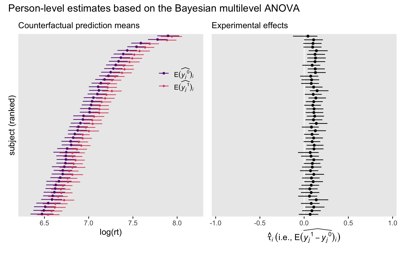
We can plot those posteriors in a figure similar to the one above.

# Counterfactual prediction means
p3 <- brm_anova_epred_i |> 
  pivot_longer(ends_with("congruent"), names_to = "cond") |> 
  mutate(y = ifelse(cond == "congruent", "E(widehat(italic(y[j])^0))[italic(i)]", "E(widehat(italic(y[j])^1))[italic(i)]")) |> 

  ggplot(aes(x = value, y = reorder(subject, rank))) +
  stat_pointinterval(aes(color = y, shape = y),
                     .width = 0.95, point_interval = mean_qi,
                     linewidth = 1/5, size = 2,
                     position = position_dodge(width = -0.35)) +
  scale_y_discrete(breaks = NULL) +
  scale_color_viridis_d(NULL, option = "A", begin = 0.3, end = 0.6,
                        labels = scales::parse_format()) +
  scale_shape_manual(NULL, values = c(20, 18),
                     labels = scales::parse_format()) +
  guides(color = guide_legend(position = "inside"),
         shape = guide_legend(position = "inside")) +
  labs(x = "log(rt)",
       y = "subject (ranked)",
       subtitle = "Counterfactual prediction means") +
  coord_cartesian(xlim = c(6.3, 8.2)) +
  theme(legend.background = element_blank(),
        legend.position.inside = c(0.85, 0.75))

# Experimental effects
p4 <- brm_anova_epred_i |> 
  ggplot(aes(x = ate_i, y = reorder(subject, rank))) +
  geom_vline(xintercept = 0, color = "white") +
  stat_pointinterval(.width = 0.95, point_interval = mean_qi,
                     linewidth = 1/4, size = 1/2) +
  scale_y_discrete(breaks = NULL) +
  labs(x = expression(hat(tau)[italic(i)]~("i.e., "*E(widehat(italic(y[j])^1-italic(y[j])^0))[italic(i)])),
       y = NULL,
       subtitle = "Experimental effects") +
  coord_cartesian(xlim = c(-0.95, 0.95))

# Combine, entitle, and display
p3 + p4 + plot_annotation(title = "Person-level estimates based on the Bayesian multilevel ANOVA")

If we work instead with the brm_anova_epred_ij that was not averaged across trial, we can also summarize the posterior distribution for the ATE.

brm_anova_ate <- brm_anova_epred_ij |> 
  group_by(.draw) |> 
  summarise(ate = mean(tau_ij))

brm_anova_ate |> 
  summarise(m = mean(ate),
            s = sd(ate),
            lwr = quantile(ate, probs = 0.025),
            upr = quantile(ate, probs = 0.975))

## # A tibble: 1 × 4
##       m      s    lwr   upr
##   <dbl>  <dbl>  <dbl> <dbl>
## 1 0.101 0.0142 0.0735 0.129

That output is the same as we’d get from avg_comparisons().

avg_comparisons(brm_anova) |> 
  get_draws() |> 
  summarise(m = mean(draw),
            s = sd(draw),
            lwr = quantile(draw, probs = 0.025),
            upr = quantile(draw, probs = 0.975)) |> 
  mutate(across(.cols = everything(), .fns = \(x) round(x, digits = 4)))

##        m      s    lwr    upr
## 1 0.1013 0.0142 0.0735 0.1287

But as with the frequentist model, these Bayesian estimates for the ATE are not identical to the posterior for \(b_1\).

as_draws_df(brm_anova) |> 
  summarise(m = mean(b_condincongruent),
            s = sd(b_condincongruent),
            lwr = quantile(b_condincongruent, probs = 0.025),
            upr = quantile(b_condincongruent, probs = 0.975))

## # A tibble: 1 × 4
##       m      s    lwr   upr
##   <dbl>  <dbl>  <dbl> <dbl>
## 1 0.100 0.0165 0.0682 0.133

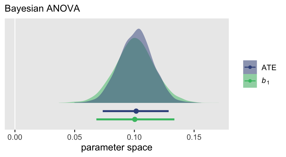
Yes, it appears they approximate one another. But very importantly, look at the precision of the estimates by their posterior \(\textit{SD}\)s and 95% intervals. The posterior for the ATE is narrower that for \(b_1\). We might further compare the two with a plot.

brm_anova_ate |> 
  rename(ATE = ate) |> 
  mutate(`italic(b)[1]` = as_draws_df(brm_anova) |> pull(b_condincongruent)) |> 
  pivot_longer(cols = -.draw) |> 
  
  ggplot(aes(x = value, fill = name, color = name)) +
  geom_vline(xintercept = 0, color = "white") +
  stat_slab(alpha = 0.5, linewidth = 0) +
  stat_pointinterval(.width = 0.95,
                     justification = 0.2, position = ggdist::position_dodgejust(width = -0.2)) +
  scale_y_continuous(NULL, breaks = NULL, expand = expansion(mult = 0.02)) +
  scale_color_viridis_d(NULL, option = "D", begin = 0.25, end = 0.7,
                        labels = scales::parse_format()) +
  scale_fill_viridis_d(NULL, option = "D", begin = 0.25, end = 0.7,
                        labels = scales::parse_format()) +
  labs(x = "parameter space",
       subtitle = "Bayesian ANOVA")

Bayesian ANCOVA and the ATE

We can compute the posteriors for the various estimands from our Bayesian ANCOVA much the same way we did for the Bayesian ANOVA, above. The only catch is to make sure the nd predictor grid has the information for the covariate[s] in the ANCOVA. In this case, it already does. We could follow all the steps above to make another version of the two-panel figure, but I’ll leave that up at an exercise for the interested reader. For many, the main goal is just to compute the posterior for \(\tau_\text{ATE}\), and perhaps compare it to the posterior for \(b_1\). Here’s the posterior for \(\tau_\text{ATE}\).

# Save
brm_ancova_ate <- avg_comparisons(brm_ancova, variables = "cond") |> 
  get_draws() |> 
  transmute(.draw = as.integer(drawid),
            ate = draw)

# Summarize
brm_ancova_ate |> 
  summarise(m = mean(ate),
            s = sd(ate),
            lwr = quantile(ate, probs = 0.025),
            upr = quantile(ate, probs = 0.975)) |> 
  mutate(across(.cols = everything(), .fns = \(x) round(x, digits = 4)))

##        m      s    lwr    upr
## 1 0.1015 0.0144 0.0732 0.1291

As with the Bayesian ANOVA, these Bayesian ANCOVA estimates for the ATE are not identical to the posterior for \(b_1\).

as_draws_df(brm_ancova) |> 
  summarise(m = mean(b_condincongruent),
            s = sd(b_condincongruent),
            lwr = quantile(b_condincongruent, probs = 0.025),
            upr = quantile(b_condincongruent, probs = 0.975))

## # A tibble: 1 × 4
##       m      s    lwr   upr
##   <dbl>  <dbl>  <dbl> <dbl>
## 1 0.101 0.0166 0.0675 0.134

Yes, they approximate one another. But the posterior for the ATE is narrower that for \(b_1\), which we might further compare the two with a plot.

brm_ancova_ate |> 
  rename(ATE = ate) |> 
  mutate(`italic(b)[1]` = as_draws_df(brm_ancova) |> pull(b_condincongruent)) |> 
  pivot_longer(cols = c(ATE, `italic(b)[1]`)) |> 
  
  ggplot(aes(x = value, fill = name, color = name)) +
  geom_vline(xintercept = 0, color = "white") +
  stat_slab(alpha = 0.5, linewidth = 0) +
  stat_pointinterval(.width = 0.95,
                     justification = 0.2, position = ggdist::position_dodgejust(width = -0.2)) +
  scale_y_continuous(NULL, breaks = NULL, expand = expansion(mult = 0.02)) +
  scale_color_viridis_d(NULL, option = "D", begin = 0.25, end = 0.7,
                        labels = scales::parse_format()) +
  scale_fill_viridis_d(NULL, option = "D", begin = 0.25, end = 0.7,
                        labels = scales::parse_format()) +
  labs(x = "parameter space",
       subtitle = "Bayesian ANCOVA")

Thus for the multilevel ANCOVA, the same pattern holds we saw for the Bayesian ANOVA. The ATE computed via g-computation has greater statistical power than the population parameter \(b_1\). If you would to make causal inferences with multilevel models, I recommend using the ATE via g-computation.

We might also go ahead and compare the ATE posteriors for the ANOVA and ANCOVA.

bind_rows(brm_anova_ate, brm_ancova_ate) |> 
  mutate(model = rep(c("ANOVA", "ANCOVA"), each = n() / 2)) |> 
  
  ggplot(aes(x = ate, fill = model, color = model)) +
  geom_vline(xintercept = 0, color = "white") +
  stat_slab(alpha = 0.5, linewidth = 0) +
  stat_pointinterval(.width = c(0.5, 0.95),
                     justification = 0.2, position = ggdist::position_dodgejust(width = -0.2)) +
  scale_y_continuous(NULL, breaks = NULL, expand = expansion(mult = 0.02)) +
  scale_color_viridis_d(NULL, option = "C", begin = 0.25, end = 0.7) +
  scale_fill_viridis_d(NULL, option = "C", begin = 0.25, end = 0.7) +
  labs(x = "ATE",
       subtitle = "Bayesian ANOVA vs Bayesian ANCOVA")

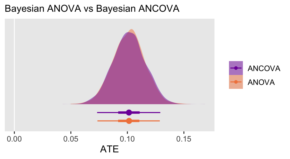
As with the frequentist models, In this case the Bayesian ANCOVA was a touch less precise than the Bayesian ANOVA, which you might find a little surprising. We’ll have more to say about this in the next post.

Wrap up

In this post, some of the main points we covered were:

• It is possible to extend the potential-outcomes framework to multilevel GLMMs.
• It is possible to fit multilevel ANOVA and ANCOVAs to data with within-person factorial designs.
• As with single-level GLMs, we generally rely on g-computation to compute the ATE.
• The \(b_1\) coefficient in a multilevel model is not the same as the ATE.
  • It appears \(b_1\) and the ATE approximate one another.
  • The ATE may be more precise than the \(b_1\) parameter, and thus has more statistical power. I say may here because though I have replicated this in other data sets, I’m not fully confident this is a general principle, and I have not yet seen rigorous methodological work on this.
• Though in some contexts the multilevel ANCOVA may improve precision on the ATE, this will not always be the case. As we will see later, there’s more than one way to fit a multilevel ANCOVA.
• Within the frequentist paradigm, the only current way to express uncertainty in the ATE is with bootstrapping. For Bayesians, there are no meaningful differences to the procedures we used for single-level GLMs.

In the next post, I plan on extending the multilevel ANOVA and ANCOVA framework for these Stroop data to consider longitudinal models, distributional models, and models with different likelihood functions. Until then, happy modeling!

Thank the reviewers

I’d like to publicly acknowledge and thank

• Vincent Arel-Bundock and
• Julia M. Rohrer

for their kind efforts reviewing the draft of this post. Go team!

Do note the final editorial decisions were my own, and I do not think it would be reasonable to assume my reviewers have given blanket endorsements of the current version of this post.

Session information

sessionInfo()

## R version 4.4.3 (2025-02-28)
## Platform: aarch64-apple-darwin20
## Running under: macOS Ventura 13.4
## 
## Matrix products: default
## BLAS:   /Library/Frameworks/R.framework/Versions/4.4-arm64/Resources/lib/libRblas.0.dylib 
## LAPACK: /Library/Frameworks/R.framework/Versions/4.4-arm64/Resources/lib/libRlapack.dylib;  LAPACK version 3.12.0
## 
## locale:
## [1] en_US.UTF-8/en_US.UTF-8/en_US.UTF-8/C/en_US.UTF-8/en_US.UTF-8
## 
## time zone: America/Chicago
## tzcode source: internal
## 
## attached base packages:
## [1] stats     graphics  grDevices utils     datasets  methods   base     
## 
## other attached packages:
##  [1] patchwork_1.3.1          marginaleffects_0.28.0.6 broom.mixed_0.2.9.5     
##  [4] tidybayes_3.0.7          brms_2.22.0              Rcpp_1.1.0              
##  [7] lme4_1.1-37              Matrix_1.7-2             lubridate_1.9.3         
## [10] forcats_1.0.0            stringr_1.5.1            dplyr_1.1.4             
## [13] purrr_1.0.4              readr_2.1.5              tidyr_1.3.1             
## [16] tibble_3.3.0             ggplot2_3.5.2            tidyverse_2.0.0         
## 
## loaded via a namespace (and not attached):
##   [1] Rdpack_2.6.2         gridExtra_2.3        inline_0.3.21       
##   [4] sandwich_3.1-1       rlang_1.1.6          magrittr_2.0.3      
##   [7] multcomp_1.4-26      furrr_0.3.1          matrixStats_1.5.0   
##  [10] compiler_4.4.3       loo_2.8.0            reshape2_1.4.4      
##  [13] vctrs_0.6.5          pkgconfig_2.0.3      arrayhelpers_1.1-0  
##  [16] fastmap_1.1.1        backports_1.5.0      labeling_0.4.3      
##  [19] utf8_1.2.6           rmarkdown_2.29       tzdb_0.4.0          
##  [22] nloptr_2.0.3         xfun_0.49            cachem_1.0.8        
##  [25] jsonlite_1.8.9       collapse_2.1.2       broom_1.0.7         
##  [28] parallel_4.4.3       R6_2.6.1             StanHeaders_2.32.10 
##  [31] bslib_0.7.0          stringi_1.8.7        RColorBrewer_1.1-3  
##  [34] parallelly_1.45.0    boot_1.3-31          jquerylib_0.1.4     
##  [37] estimability_1.5.1   bookdown_0.40        rstan_2.32.7        
##  [40] knitr_1.49           zoo_1.8-12           bayesplot_1.13.0    
##  [43] splines_4.4.3        timechange_0.3.0     tidyselect_1.2.1    
##  [46] rstudioapi_0.16.0    dichromat_2.0-0.1    abind_1.4-8         
##  [49] yaml_2.3.8           codetools_0.2-20     blogdown_1.20       
##  [52] curl_6.0.1           pkgbuild_1.4.8       listenv_0.9.1       
##  [55] plyr_1.8.9           lattice_0.22-6       withr_3.0.2         
##  [58] bridgesampling_1.1-2 posterior_1.6.1      coda_0.19-4.1       
##  [61] evaluate_1.0.1       future_1.58.0        survival_3.8-3      
##  [64] RcppParallel_5.1.10  ggdist_3.3.2         pillar_1.11.0       
##  [67] tensorA_0.36.2.1     checkmate_2.3.2      stats4_4.4.3        
##  [70] insight_1.3.1        reformulas_0.4.1     distributional_0.5.0
##  [73] generics_0.1.4       hms_1.1.3            rstantools_2.4.0    
##  [76] scales_1.4.0         minqa_1.2.6          globals_0.18.0      
##  [79] xtable_1.8-4         glue_1.8.0           emmeans_1.10.3      
##  [82] tools_4.4.3          data.table_1.17.8    mvtnorm_1.3-3       
##  [85] grid_4.4.3           QuickJSR_1.8.0       rbibutils_2.3       
##  [88] colorspace_2.1-1     nlme_3.1-167         cli_3.6.5           
##  [91] svUnit_1.0.6         viridisLite_0.4.2    Brobdingnag_1.2-9   
##  [94] V8_4.4.2             gtable_0.3.6         sass_0.4.9          
##  [97] digest_0.6.37        TH.data_1.1-2        farver_2.1.2        
## [100] htmltools_0.5.8.1    lifecycle_1.0.4      MASS_7.3-64

References

Arel-Bundock, V. (2023). marginaleffects: Predictions, Comparisons, Slopes, Marginal Means, and Hypothesis Tests [Manual]. [https://vincentarelbundock.github.io/ marginaleffects/ https://github.com/vincentarelbundock/ marginaleffects]( https://vincentarelbundock.github.io/ marginaleffects/ https://github.com/vincentarelbundock/ marginaleffects)
Bates, D., Maechler, M., Bolker, B., & Steven Walker. (2022). lme4: Linear mixed-effects models using Eigen’ and S4. https://CRAN.R-project.org/package=lme4
Bolker, B., & Robinson, D. (2022). broom.mixed: Tidying methods for mixed models [Manual]. https://github.com/bbolker/broom.mixed
Brooks, M., Bolker, B., Kristensen, K., Maechler, M., Magnusson, A., Skaug, H., Nielsen, A., Berg, C., & van Bentham, K. (2023). glmmTMB: Generalized linear mixed models using template model builder [Manual]. https://github.com/glmmTMB/glmmTMB
Brumback, B. A. (2022). Fundamentals of causal inference with R. Chapman & Hall/CRC. https://www.routledge.com/Fundamentals-of-Causal-Inference-With-R/Brumback/p/book/9780367705053
Bürkner, P.-C. (2017). brms: An R package for Bayesian multilevel models using Stan. Journal of Statistical Software, 80(1), 1–28. https://doi.org/10.18637/jss.v080.i01
Bürkner, P.-C. (2018). Advanced Bayesian multilevel modeling with the R package brms. The R Journal, 10(1), 395–411. https://doi.org/10.32614/RJ-2018-017
Bürkner, P.-C. (2022). brms: Bayesian regression models using ’Stan’. https://CRAN.R-project.org/package=brms
Collins, L. M. (2006). Analysis of longitudinal data: The integration of theoretical model, temporal design, and statistical model. Annual Review of Psychology, 57(1), 505–528. https://doi.org/10.1146/annurev.psych.57.102904.190146
Cooper, J. O., Heron, T. E., & Heward, W. L. (2019). Applied behavior analysis (Third Edition). Pearson Education. https://www.pearson.com/
Cunningham, S. (2021). Causal inference: The mixtape. Yale University Press. https://mixtape.scunning.com/
Demšar, J., Repovš, G., & Štrumbelj, E. (2023). Bayes4psy: User friendly bayesian data analysis for psychology [Manual]. https://CRAN.R-project.org/package=bayes4psy
Faraway, J. J. (2016). Extending the linear model with R: Generalized linear, mixed effects and nonparametric regression models (Second Edition). Chapman and Hall/CRC. https://julianfaraway.github.io/faraway/ELM/
Feller, A., & Gelman, A. (2015). Hierarchical models for causal effects. In R. A. Scott & M. C. Buchmann (Eds.), Emerging trends in the social and behavioral sciences (pp. 1–16). John Wiley & Sons, Ltd. https://onlinelibrary.wiley.com/doi/book/10.1002/9781118900772
Gelman, A., & Hill, J. (2006). Data analysis using regression and multilevel/hierarchical models. Cambridge University Press. https://doi.org/10.1017/CBO9780511790942
Hernán, M. A., & Robins, J. M. (2020). Causal inference: What if. Boca Raton: Chapman & Hall/CRC. https://www.hsph.harvard.edu/miguel-hernan/causal-inference-book/
Hill, J. (2013). Multilevel models and causal inference. In M. A. Scott, J. S. Simonoff, & B. D. Marx (Eds.), The SAGE handbook of multilevel modeling (pp. 201–220). SAGE Publications Ltd. https://us.sagepub.com/en-us/nam/the-sage-handbook-of-multilevel-modeling/book235673
Holland, P. W. (1986). Statistics and causal inference. Journal of the American Statistical Association, 81(396), 945–960. https://doi.org/ https://dx.doi.org/10.1080/01621459.1986.10478354
Imbens, G. W., & Rubin, D. B. (2015). Causal inference in statistics, social, and biomedical sciences: An Introduction. Cambridge University Press. https://doi.org/10.1017/CBO9781139025751
Kay, M. (2021). ggdist: Visualizations of distributions and uncertainty [Manual]. https://CRAN.R-project.org/package=ggdist
Kay, M. (2023). tidybayes: Tidy data and ’geoms’ for Bayesian models. https://CRAN.R-project.org/package=tidybayes
Kazdin, A. E. (2017). Research design in clinical psychology, 5th Edition. Pearson. https://www.pearson.com/
Kruschke, J. K. (2015). Doing Bayesian data analysis: A tutorial with R, JAGS, and Stan. Academic Press. https://sites.google.com/site/doingbayesiandataanalysis/
MacLeod, C. M. (1991). Half a century of research on the Stroop effect: An integrative review. Psychological Bulletin, 109(2), 163–203. https://doi.org/10.1037/0033-2909.109.2.163
Martin, S. R. (2020). Is the LKJ(1) prior uniform? “Yes”. https://srmart.in/is-the-lkj1-prior-uniform-yes/
McElreath, R. (2015). Statistical rethinking: A Bayesian course with examples in R and Stan. CRC press. https://xcelab.net/rm/statistical-rethinking/
McElreath, R. (2020). Statistical rethinking: A Bayesian course with examples in R and Stan (Second Edition). CRC Press. https://xcelab.net/rm/statistical-rethinking/
Pedersen, T. L. (2022). patchwork: The composer of plots. https://CRAN.R-project.org/package=patchwork
R Core Team. (2025). R: A language and environment for statistical computing. R Foundation for Statistical Computing. https://www.R-project.org/
Raudenbush, S. W., & Schwartz, D. (2020). Randomized experiments in education, with implications for multilevel causal inference. Annual Review of Statistics and Its Application, 7(1), 177–208. https://doi.org/10.1146/annurev-statistics-031219-041205
Roback, P., & Legler, J. (2021). Beyond multiple linear regression: Applied generalized linear models and multilevel models in R. CRC Press. https://bookdown.org/roback/bookdown-BeyondMLR/
Robins, J. (1986). A new approach to causal inference in mortality studies with a sustained exposure period—application to control of the healthy worker survivor effect. Mathematical Modelling, 7(9–12), 1393–1512. https://doi.org/10.1016/0270-0255(86)90088-6
Senn, S. S. (2002). Cross-over trials in clinical research. John Wiley & Sons. https://doi.org/10.1002/0470854596
Shadish, W. R., Cook, T. D., & Campbell, D. T. (2002). Experimental and quasi-experimental designs for generalized causal inference. Houghton, Mifflin and Company.
Snodgrass, J. G., Luce, R. D., & Galanter, E. (1967). Some experiments on simple and choice reaction time. Journal of Experimental Psychology, 75(1), 1. https://doi.org/10.1037/h0021280
Stroop, J. R. (1935). Studies of interference in serial verbal reactions. Journal of Experimental Psychology, 18(6), 643. https://doi.org/10.1037/h0054651
Taback, N. (2022). Design and analysis of experiments and observational studies using R. Chapman and Hall/CRC. https://doi.org/10.1201/9781003033691
Wickham, H. (2022). tidyverse: Easily install and load the ’tidyverse’. https://CRAN.R-project.org/package=tidyverse
Wickham, H., Averick, M., Bryan, J., Chang, W., McGowan, L. D., François, R., Grolemund, G., Hayes, A., Henry, L., Hester, J., Kuhn, M., Pedersen, T. L., Miller, E., Bache, S. M., Müller, K., Ooms, J., Robinson, D., Seidel, D. P., Spinu, V., … Yutani, H. (2019). Welcome to the tidyverse. Journal of Open Source Software, 4(43), 1686. https://doi.org/10.21105/joss.01686
Wikipedia contributors. (2025, July 20). Stroop effect. https://en.wikipedia.org/wiki/Stroop_effect
-
Or series of series, I suppose… ↩︎
I’m presuming it was online, anyways. The documentation from
?bayes4psy::stroop_extendedwasn’t as specific as I would have hoped. You get what you pay for, friends. ↩︎ -
See this GitHub issue for updates on this. ↩︎
Or at least, as simple as we can given the context. ↩︎
Though we do not do so here, it is possible to relax this constraint in various ways. Frequentists can do so to some degree with the glmmTMB package ( Brooks et al., 2023). ↩︎
Keep in mind the basic interpretation for a regression interpretation is it is the change in the expected value for the DV, given a one-unit increase in the predictor variable for the coefficient. Thus if your predictor variables have wide ranges, one-unit increases probably won’t have a big change in expectation for the DV. But if your predictor variables have small ranges, a one-unit increase might well make for a massive difference in DV expectation. ↩︎
We’ll do better in a future post. ↩︎
Often the control or baseline condition. ↩︎
Often the experimental or contrasting condition. ↩︎
Different research traditions use different terms for such things. I’m borrowing the term intensive longitudinal from the daily-diary research tradition in psychology, where people typically answer a few questions once or a few times a day for several days or weeks (see Collins, 2006). Comparatively, you might describe reaction-time data from computer tasks as very intensive longitudinal data. ↩︎
I should add that to my knowledge this insight is largely missing from the formal methodological literature, and conflicts somewhat from some of the published work, such as Raudenbush & Schwartz ( 2020). I bet this would make for a great dissertation topic for a grad student in, say, quantitative psychology or perhaps statistics. If you decide to take it on, just make sure to cite uncle Solomon’s blog post, and tell me all about your exciting results so I can share them with my readers. ↩︎
Before you try this on your own computer, make sure you’re using marginaleffects version 0.28.0.6 or higher. If you need it, you can install the current developmental version by executing
remotes::install_github("vincentarelbundock/marginaleffects", force = TRUE). ↩︎ -
Yeah, I’ll admit it. Those intervals look surprisingly janky and asymmetrical to my eye. The last time I dove seriously into the bootstrapping literature was the early 2000 teens when I and all of my colleagues were learning about BCa CIs for mediation analyses. I wasn’t even into Bayes yet. I did a casual survey of some of the bootstrapping literature for multilevel models in preparation for this post, and my impression was the methods available by
inferences()are generally fine for many use cases. However, if any of y’all readers are bootstrap jocks with important insights for this application, share them in the comments. ↩︎ -
We’ll have more to say about this later. ↩︎
- Posted on:
- July 20, 2025
- Length:
- 52 minute read, 10927 words