Learn Stan with brms, Part III
y ~ 1 + x
By A. Solomon Kurz
July 17, 2025
Center the \(x\)
In the last post, we fit a model with a single continuous predictor using the very non-default brms syntax bf(y ~ 1 + x, center = FALSE). We also had some difficulty settling on a sensible prior for the intercept in this context, given how all our predictor values were far above zero. In this post we’ll explore different ways to fit the model with a mean-centered predictor, what this means for how we set our priors with brms, and what this all means for the underlying Stan code. Along the way we practice with the transformed data block, and get fancier with the model matrix.
Load the primary R packages and the data file.
# Packages
library(tidyverse)
library(brms)
library(rstan)
library(tidybayes)
library(ggdist)
library(posterior)
library(patchwork)

# Data
load(file = "data/d.rda")

# Review
glimpse(d)
## Rows: 100
## Columns: 3
## $ male   <dbl> 0, 1, 0, 1, 1, 0, 0, 0, 1, 0, 0, 0, 0, 0, 0, 1, 0, 0, 1, 1, 0, …
## $ height <dbl> 63.9, 68.0, 63.9, 70.1, 72.5, 64.2, 61.9, 62.1, 74.9, 63.5, 63.…
## $ weight <dbl> 141.7, 210.1, 162.5, 138.2, 193.8, 155.3, 197.8, 147.4, 178.9, …
We continue with the height and weight data. For the code underlying the data, review the appendix from the first post.
Focal model
In this post we will fit the univariable model
$$
\begin{align} \text{weight}_i & \sim \operatorname{Normal}(\mu_i, \sigma) \\ \mu_i & = \beta_0 + \beta_1 \text{height}_i \\ \beta_0 & \sim \mathord ? \\ \beta_1 & \sim \operatorname{Normal}(5, 2.5) \\ \sigma & \sim \operatorname{Exponential}(0.04), \end{align}
$$
where weight values vary across \(i\) people, and they are modeled as normally distributed with a conditional mean \(\mu_i\) and [residual] standard deviation \(\sigma\). The conditional mean is defined by an intercept \(\beta_0\) and slope \(\beta_1\) for the predictor variable height.
That’s the same model as last time, you say. Well, yes and no. In another sense, we’ll also be fitting the model
$$
\begin{align} \text{weight}_i & \sim \operatorname{Normal}(\mu_i, \sigma) \\ \mu_i & = \beta_0 + \beta_1 \left ( \text{height}_i - \overline{\text{height}} \right ) \\ \beta_0 & \sim \mathord ? \\ \beta_1 & \sim \operatorname{Normal}(5, 2.5) \\ \sigma & \sim \operatorname{Exponential}(0.04), \end{align}
$$
where \(\overline{\text{height}}\) is the sample mean for height, and \((\text{height}_i - \overline{\text{height}})\) is mean-centered height. But wait; which one are we fitting? you ask. In a way, we’ll be fitting both.
As to the priors, you may have noticed two things. First, there’s a big question mark by the intercept \(\beta_0\), which is my way of indicating we’re not ready to discuss that prior, yet. But otherwise you may have also noticed the priors for \(\beta_1\) and \(\sigma\) are the same as in the last post. Before we can fully discuss the prior for \(\beta_0\), we need to discuss how brms handles mean-centering predictors.
brms workflow
brm() automatically mean centers your predictors
Read that header again. Unless you tell it otherwise, the brm() function automatically mean centers your predictors. After mean centering the predictors, it then fits the model with those centered predictors as the inputs. This has no effect on the coefficients for the predictors themselves (the regression slopes), but is has a profound effect on the “intercept.” At this point, we should probably quote from the
brms Reference Manual (
Bürkner, 2024) at length. Here’s the Parameterization of the population-level intercept section, in full:
By default, the population-level intercept (if incorporated) is estimated separately and not as part of population-level parameter vector
b. As a result, priors on the intercept also have to be specified separately. Furthermore, to increase sampling efficiency, the population-level design matrixXis centered around its column meansX_meansif the intercept is incorporated. This leads to a temporary bias in the intercept equal to<X_means, b>, where<,>is the scalar product. The bias is corrected after fitting the model, but be aware that you are effectively defining a prior on the intercept of the centered design matrix not on the real intercept. You can turn off this special handling of the intercept by setting argumentcentertoFALSE. For more details on setting priors on population-level intercepts, seeset_prior.This behavior can be avoided by using the reserved (and internally generated) variable
Intercept. Instead ofy ~ x, you may writey ~ 0 + Intercept + x. This way, priors can be defined on the real intercept, directly. In addition, the intercept is just treated as an ordinary population-level effect and thus priors defined onbwill also apply to it. Note that this parameterization may be less efficient than the default parameterization discussed above.
As indicated in the first paragraph, this has consequences for how you set your priors. From the set_prior section, we read:
In case of the default intercept parameterization (discussed in the ‘Details’ section of
brmsformula), general priors on class"b"will not affect the intercept. Instead, the intercept has its own parameter class named"Intercept"and priors can thus be specified viaset_prior("<prior>", class = "Intercept"). Setting a prior on the intercept will not break vectorization of the other population-level effects. Note that technically, this prior is set on an intercept that results when internally centering all population-level predictors around zero to improve sampling efficiency. On this centered intercept, specifying a prior is actually much easier and intuitive than on the original intercept, since the former represents the expected response value when all predictors are at their means. To treat the intercept as an ordinary population-level effect and avoid the centering parameterization, use0 + Intercepton the right-hand side of the model formula.
To understand what this all means in practice, consider a scenario where you’d like to fit the model y ~ 1 + x, where the predictor x is not mean centered (such as in our case with height). If you would like to set the prior for \(\beta_0\) given a non-centered predictor, you can use one of these two strategies:
# The `bf(center = FALSE)` method
brm(
  ...,
  bf(y ~ 1 + x, center = FALSE),
  prior = prior(normal(<mean>, <sd>), class = b, coef = Intercept),
  ...)

# The `0 + Intercept` method
brm(
  ...,
  y ~ 0 + Intercept + x,
  prior = prior(normal(<mean>, <sd>), class = b, coef = Intercept),
  ...)
The first strategy sets center = FALSE within the bf() function, and the second strategy uses the 0 + Intercept syntax. In both cases, when you set the prior for \(\beta_0\), it is of class = b and coef = Intercept. The first of these two options is what we did for brm2 from the
last post. The relevant bit of code was:
brm(
  ...,
  bf(weight ~ 1 + height, center = FALSE),
  prior = prior(normal(0, 100), class = b, coef = Intercept),
  ...)
However, if you would like to set the prior for \(\beta_0\) as if you were using a mean-centered predictor and therefore \(\beta_0\) was “the expected response value when all predictors are at their means,” then you can use the simpler default syntax of:
# The default method
brm(
  ...,
  y ~ 1 + x,
  prior = prior(normal(<mean>, <sd>), class = Intercept),
  ...)
But do keep in mind that the \(\beta_0\) intercept under this prior is not the \(\beta_0\) coefficient displayed in the print() summary. Rather, that \(\beta_0\) coefficient is computed “after fitting the model,” which we will demonstrate below with the stan() versions of the model. This will be our approach here. One of Bürkner’s claims in the quotes above was “specifying a prior is actually much easier and intuitive [on this centered intercept] than on the original intercept, since the former represents the expected response value when all predictors are at their means.” To get a sense of what that means for our use case, here’s the model we’ll fit:
$$
\begin{align} \text{weight}_i & \sim \operatorname{Normal}(\mu_i, \sigma) \\ \mu_i & = \beta_0 + \beta_1 \left ( \text{height}_i - \overline{\text{height}} \right ) \\ \beta_0 & \sim \operatorname{Normal}(160, 25) \\ \beta_1 & \sim \operatorname{Normal}(5, 2.5) \\ \sigma & \sim \operatorname{Exponential}(0.04), \end{align}
$$
where even though we’re entering height into the formula in brm(), we know that under the hood it’s actually using \((\text{height}_i - \overline{\text{height}})\). The \(\operatorname{Normal}(160, 25)\) prior for \(\beta_0\) given the mean-centered predictor is the same prior we used for the unconditional mean in brm1, the model from the
first post. As a general strategy, whatever prior you would use for an unconditional mean, I suspect that would also be a good prior for a model conditional on mean-centered predictors.
Fit the model with brm()
Here’s how to fit the model with brm(). Note how since we are using the simple y ~ 1 + x syntax, the prior for \(\beta_0\) is simply of class = Intercept.
brm3 <- brm(
  data = d,
  weight ~ 1 + height,
  prior = prior(normal(160, 25), class = Intercept) +
    prior(normal(5, 2.5), class = b) +
    prior(exponential(0.04), class = sigma),
  cores = 4, seed = 1,
  file = "fits/brm3")
Review the print() summary.
print(brm3)
##  Family: gaussian
##   Links: mu = identity; sigma = identity
## Formula: weight ~ 1 + height
##    Data: d (Number of observations: 100)
##   Draws: 4 chains, each with iter = 2000; warmup = 1000; thin = 1;
##          total post-warmup draws = 4000
##
## Regression Coefficients:
##           Estimate Est.Error l-95% CI u-95% CI Rhat Bulk_ESS Tail_ESS
## Intercept   -80.59     45.91  -170.19    10.77 1.00     3552     2557
## height        3.58      0.69     2.21     4.93 1.00     3516     2617
##
## Further Distributional Parameters:
##       Estimate Est.Error l-95% CI u-95% CI Rhat Bulk_ESS Tail_ESS
## sigma    28.91      2.07    25.19    33.31 1.00     3645     2796
##
## Draws were sampled using sampling(NUTS). For each parameter, Bulk_ESS
## and Tail_ESS are effective sample size measures, and Rhat is the potential
## scale reduction factor on split chains (at convergence, Rhat = 1).
The summaries for \(\beta_1\) and \(\sigma\) are about the same as they were for brm2 from the
second post. The Intercept line is a summary for the intercept had you fit the model with the non-mean centered version of the predictor height. There is no summary of the actual intercept brm() used internally to fit the model from print(), but we do still have access to that parameter. Behold the summary from the posterior_summary() function:
posterior_summary(brm3)
##               Estimate  Est.Error        Q2.5       Q97.5
## b_Intercept  -80.58762 45.9075910 -170.191525   10.766353
## b_height       3.57804  0.6902908    2.214516    4.933541
## sigma         28.90547  2.0693197   25.185225   33.310604
## Intercept    156.65071  2.9021135  150.783782  162.225007
## lprior       -10.56372  0.1895477  -11.026650  -10.287216
## lp__        -485.48535  1.2513430 -488.721443 -484.076025
Confusingly, the top row b_Intercept here is the same as the row called Intercept in the print() output. The new line called Intercept is the intercept for the model using mean-centered height. Notice how that value is about the same as the unconditional mean from brm1 from the
first post,1 and that value is pretty close to where we centered our prior.
You also get the same parameter-name convention in functions like as_draws_df().
draws_brm3 <- as_draws_df(brm3)  # Compute and save
glimpse(draws_brm3)              # Display
## Rows: 4,000
## Columns: 9
## $ b_Intercept <dbl> -9.860513, -40.876677, -101.749180, -34.797674, -97.383514…
## $ b_height    <dbl> 2.518596, 2.984522, 3.917371, 2.928780, 3.861822, 3.994814…
## $ sigma       <dbl> 28.58365, 32.76419, 25.15680, 35.09813, 31.98618, 29.57765…
## $ Intercept   <dbl> 157.1325, 157.0091, 157.9882, 159.3921, 158.6707, 158.2150…
## $ lprior      <dbl> -10.83443, -10.83462, -10.29520, -10.93934, -10.57642, -10…
## $ lp__        <dbl> -485.1696, -486.1156, -485.9663, -488.5022, -485.5042, -48…
## $ .chain      <int> 1, 1, 1, 1, 1, 1, 1, 1, 1, 1, 1, 1, 1, 1, 1, 1, 1, 1, 1, 1…
## $ .iteration  <int> 1, 2, 3, 4, 5, 6, 7, 8, 9, 10, 11, 12, 13, 14, 15, 16, 17,…
## $ .draw       <int> 1, 2, 3, 4, 5, 6, 7, 8, 9, 10, 11, 12, 13, 14, 15, 16, 17,…
The first column b_Intercept is the intercept had you fit the model with non-mean-centered height, and the fourth column Intercept is the parameter we actually set the prior on, the intercept given mean-centered height.
To further illustrate this whole confusing mess, let’s make a plot.
xmax <- max(d$height) |> ceiling()
ymax <- max(d$weight)
ymin <- as_draws_df(brm3) |> summarise(quantile(b_Intercept, 0.025)) |> pull()
m_x <- mean(d$height)
m_y <- mean(d$weight)

# Left
p1 <- data.frame(height = 0:xmax) |>
  add_epred_draws(brm3) |>
  rename(weight = .epred) |>

  ggplot(aes(x = height, y = weight)) +
  geom_hline(yintercept = m_y, color = "white") +
  geom_vline(xintercept = m_x, color = "white") +
  stat_lineribbon(.width = 0.95,
                  color = "steelblue4", fill = "steelblue1", linewidth = 1/2) +
  geom_point(data = d) +
  coord_cartesian(ylim = c(ymin, ymax)) +
  theme(panel.grid = element_blank())

# Right
p2 <- draws_brm3 |>
  pivot_longer(cols = contains("Intercept")) |>

  ggplot(aes(y = value, x = name)) +
  geom_hline(yintercept = m_y, color = "white") +
  stat_pointinterval(.width = 0.95,
               color = "steelblue4", size = 1/10) +
  scale_x_discrete(NULL, position = "top") +
  scale_y_continuous(NULL, breaks = NULL, limits = c(ymin, ymax)) +
  theme(axis.text.x = element_text(angle = 270, hjust = 1),
        panel.grid = element_blank())

# Combine, format, and display
p1 + p2 +
  plot_layout(widths = c(15, 1))
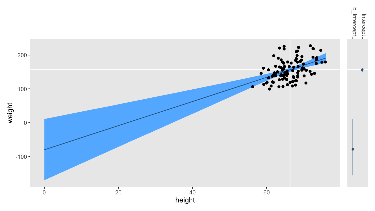
In the main panel on the left, you have the fitted line which looks a lot like the one from the
second post. The white lines intersecting in the middle of the data cloud mark off the sample means for height and weight. Now notice the skinny coefficient plot in the right panel. See the wide point interval toward the bottom? That marks of the version of \(\beta_0\) called b_Intercept in the posterior_summary() and as_draws_df() output; that’s the intercept had we fit the model using height. But notice the point interval for the Intercept coefficient. That’s the one for the intercept with the model fit to mean-centered height, and that’s the coefficient for which we set the prior prior(normal(160, 25), class = Intercept).
Real talk
In my opinion, this was easily the worst programming decision Bürkner made for brms. I hate it that when I enter y ~ 1 + x in the formula line, I’m asked to set the intercept prior based on y ~ 1 + (x - mean(x)) as a default. It’s inherently confusing, and the way that print() and posterior_summary() use different naming conventions for the intercept makes it worse. I’d bet a lot of brms users don’t even understand this, which makes me suspect that several folks may have published scientific articles based on models fit using the wrong intercept priors. It’s a disaster.
If you want to avoid all this, either set center = FALSE, or use the 0 + Intercept syntax. This is what I do most of the time for my real-world projects. When I want to fit a model with mean-centered predictors (which I sometimes do), I prefer centering them myself. But the brms Reference Manual said this was all to “increase sampling efficiency,” you say. I do not care. Personally, I would much rather take a little longer during the sampling phase than risk incorrectly setting a prior out of syntax confusion.
However, since this is what brms() does, we can at least work to understand it further by diving into the underlying Stan code, and reproducing the results with stan(). But before we do, let’s practice a little algebra.
Compute b_Intercept from Intercept, by hand
We can compute \(\beta_0\) using the equation
$$ \beta_0 = \beta_{0_\text{temporary}} - \overline{\text{height}} \beta_1 $$
where \(\overline{\text{height}}\) is the sample mean for height, and \(\beta_1\) is the regression coefficient for height. With this notation, I’m calling the intercept for height \(\beta_0\), and the intercept for mean-centered height \(\beta_{0_\text{temporary}}\). In the as_draws_df() output, these are b_Intercept and Intercept, respectively.
Here’s what this algebra can look like in code. We’ll plot the results.
draws_brm3 |>
  # Use the equation
  mutate(`Intercept - m_x * b_height` = Intercept - m_x * b_height) |>
  pivot_longer(cols = c(b_Intercept, `Intercept - m_x * b_height`)) |>

  # Plot
  ggplot(aes(x = value, y = name)) +
  stat_halfeye(.width = 0.95) +
  scale_y_discrete(NULL, expand = expansion(mult = 0.1)) +
  xlab(expression(beta[0])) +
  theme(panel.grid = element_blank())
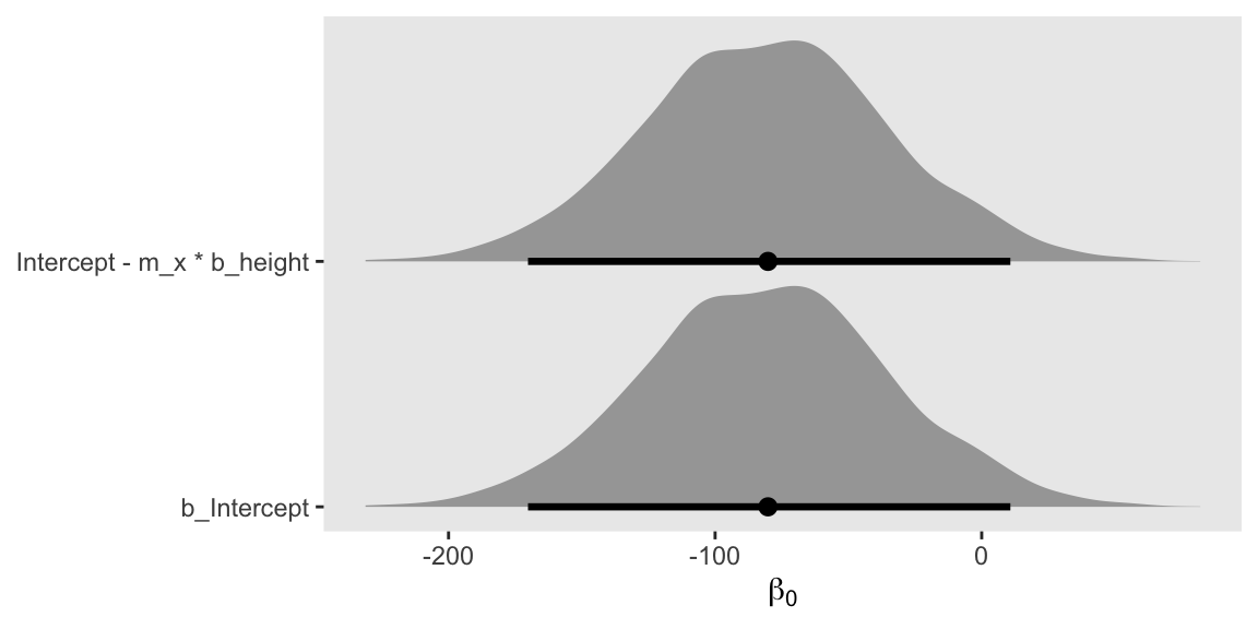
Are they identical?
draws_brm3 |>
  mutate(b_Intercept_by_hand = Intercept - (m_x * b_height)) |>
  summarise(all_equal = all.equal(b_Intercept, b_Intercept_by_hand))
## # A tibble: 1 × 1
##   all_equal
##   <lgl>
## 1 TRUE
Yes. We’ll see more of that algebra in action in the Stan code below.
Extract the Stan code with stancode()
Extract the Stan code underlying our brm3 model with the stancode() function.
stancode(brm3)
## // generated with brms 2.22.0
## functions {
## }
## data {
##   int<lower=1> N;  // total number of observations
##   vector[N] Y;  // response variable
##   int<lower=1> K;  // number of population-level effects
##   matrix[N, K] X;  // population-level design matrix
##   int<lower=1> Kc;  // number of population-level effects after centering
##   int prior_only;  // should the likelihood be ignored?
## }
## transformed data {
##   matrix[N, Kc] Xc;  // centered version of X without an intercept
##   vector[Kc] means_X;  // column means of X before centering
##   for (i in 2:K) {
##     means_X[i - 1] = mean(X[, i]);
##     Xc[, i - 1] = X[, i] - means_X[i - 1];
##   }
## }
## parameters {
##   vector[Kc] b;  // regression coefficients
##   real Intercept;  // temporary intercept for centered predictors
##   real<lower=0> sigma;  // dispersion parameter
## }
## transformed parameters {
##   real lprior = 0;  // prior contributions to the log posterior
##   lprior += normal_lpdf(b | 5, 2.5);
##   lprior += normal_lpdf(Intercept | 160, 25);
##   lprior += exponential_lpdf(sigma | 0.04);
## }
## model {
##   // likelihood including constants
##   if (!prior_only) {
##     target += normal_id_glm_lpdf(Y | Xc, Intercept, b, sigma);
##   }
##   // priors including constants
##   target += lprior;
## }
## generated quantities {
##   // actual population-level intercept
##   real b_Intercept = Intercept - dot_product(means_X, b);
## }
A lot of this stuff should look familiar at this point. But there are a few new features scattered throughout several of the blocks.
Extract the Stan data with standata()
Investigate the data brms actually passed onto Stan with the standata() function.
standata(brm3) |>
  str()
## List of 6
##  $ N         : int 100
##  $ Y         : num [1:100(1d)] 142 210 162 138 194 ...
##  $ K         : int 2
##  $ Kc        : num 1
##  $ X         : num [1:100, 1:2] 1 1 1 1 1 1 1 1 1 1 ...
##   ..- attr(*, "dimnames")=List of 2
##   .. ..$ : chr [1:100] "1" "2" "3" "4" ...
##   .. ..$ : chr [1:2] "Intercept" "height"
##   ..- attr(*, "assign")= int [1:2] 0 1
##  $ prior_only: int 0
##  - attr(*, "class")= chr [1:2] "standata" "list"
We have seen all of these features before.2
rstan workflow
This time we will only fit two models. We’ll start very simple with stan3.1, and finish by implementing all the new features with stan3.2.
stan3.1, start as simple as one can
First, we define the data list with compose_data().
stan_data <- d |>
  select(weight, height) |>
  compose_data()

str(stan_data)
## List of 3
##  $ weight: num [1:100(1d)] 142 210 162 138 194 ...
##  $ height: num [1:100(1d)] 63.9 68 63.9 70.1 72.5 64.2 61.9 62.1 74.9 63.5 ...
##  $ n     : int 100
For this version of the data, we only need the weight and height values as vectors, and the only scalar necessary is n.
We can define the simplest version of the model_code like so.
model_code_3.1 <- '
data {
  int<lower=1> n;
  vector[n] weight;
  vector[n] height;
}
transformed data {
  real mean_height = mean(height);            // Sample mean for the predictor
  vector[n] height_c = height - mean_height;  // Mean-centered version of the predictor
}
parameters {
  real beta0_c;  // Temporary intercept for centered predictors
  real beta1;
  real<lower=0> sigma;
}
model {
  weight ~ normal(beta0_c + beta1 * height_c, sigma);  // Likelihood
  beta0_c ~ normal(160, 25);                           // Priors
  beta1 ~ normal(5, 2.5);
  sigma ~ exponential(0.04);
}
generated quantities {
  // Compute the actual intercept for the model using the non-centered predictor
  real beta0 = beta0_c - mean_height * beta1;
}
'
Of note, we have two lines in our transformed data block. The first line computes the mean of the height vector, and saves that quantity as a real value named mean_height. The second line subtracts the mean_height value from each row in the height vector, and saves it as a new vector named height_c, the _c suffix for which stands for centered.
The beta1 and sigma parameters in our parameters block are business-as-usual at this point. The first line, however, defines beta0_c as the “Temporary intercept for centered predictors.”
Next focus on the model block. In the likelihood line we use the height_c vector as the predictor which is multiplied with beta1, and the beta0_c parameter serves as the intercept. The normal(160, 25) prior is applied to the temporary beta0_c intercept, and the other two priors are used in the usual way.
Finally notice the generated quantities block. There we use the equation from
above to compute beta0, which is the intercept for the model had it been fit with the non-centered vector height. Recall that because it is defined in the generated quantities, the beta0 parameter is computed after the HMC samples are completed.
Fit the model with stan().
stan3.1 <- stan(
  data = stan_data,
  model_code = model_code_3.1,
  cores = 4, seed = 1)
Now we check the model summary. Here we’ll compare it directly with the posterior_summary() summary for brm3, as also shown above.
# print(brm3)
posterior_summary(brm3) |>
  round(digits = 2)
##             Estimate Est.Error    Q2.5   Q97.5
## b_Intercept   -80.59     45.91 -170.19   10.77
## b_height        3.58      0.69    2.21    4.93
## sigma          28.91      2.07   25.19   33.31
## Intercept     156.65      2.90  150.78  162.23
## lprior        -10.56      0.19  -11.03  -10.29
## lp__         -485.49      1.25 -488.72 -484.08
print(stan3.1, probs = c(0.025, 0.975))
## Inference for Stan model: anon_model.
## 4 chains, each with iter=2000; warmup=1000; thin=1;
## post-warmup draws per chain=1000, total post-warmup draws=4000.
##
##            mean se_mean    sd    2.5%   97.5% n_eff Rhat
## beta0_c  156.67    0.05  2.91  150.98  162.45  3624    1
## beta1      3.56    0.01  0.70    2.20    4.95  4422    1
## sigma     28.96    0.03  2.10   25.29   33.41  3654    1
## beta0    -79.56    0.70 46.37 -170.84   11.38  4440    1
## lp__    -384.42    0.03  1.28 -387.74 -383.00  1987    1
##
## Samples were drawn using NUTS(diag_e) at Thu Jul 17 14:24:30 2025.
## For each parameter, n_eff is a crude measure of effective sample size,
## and Rhat is the potential scale reduction factor on split chains (at
## convergence, Rhat=1).
The summaries overlap nicely. What the stan3.1 output calls beta0_c and beta0, the brm3 output calls Intercept and b_Intercept.
stan3.2 for new tricks and the final model
For the data list, add the prior_only value and the model matrix.
mm3.2 <- model.matrix(data = d, object = ~height)

stan_data <- d |>
  select(weight) |>
  compose_data(k = ncol(mm3.2),
               kc = ncol(mm3.2) - 1,
               X = mm3.2,
               prior_only = as.integer(FALSE))

str(stan_data, give.attr = FALSE)
## List of 6
##  $ weight    : num [1:100(1d)] 142 210 162 138 194 ...
##  $ n         : int 100
##  $ k         : int 2
##  $ kc        : num 1
##  $ X         : num [1:100, 1:2] 1 1 1 1 1 1 1 1 1 1 ...
##  $ prior_only: int 0
Note how we now define the total number of columns in the model matrix as k, and kc is one minus that value. We subtract one because the kc value is excluding the vector of 1’s for the intercept, which we’ll explain in more detail later.
Here’s how to make the full version of the model_code.
model_code_3.2 <- '
data {
  int<lower=1> n;
  int<lower=1> k;   // Number of beta coefficients in the linear model
  int<lower=1> kc;  // number of beta coefficients minus the intercept
  vector[n] weight;
  matrix[n, k] X;
  int prior_only;
}
transformed data {
  matrix[n, kc] Xc;    // Centered version of X without an intercept
  vector[kc] means_X;  // Column means of X before centering
  for (i in 2:k) {
    means_X[i - 1] = mean(X[, i]);
    Xc[, i - 1] = X[, i] - means_X[i - 1];
  }
}
parameters {
  vector[kc] b;    // Beta coefficients (minus the intercept)
  real Intercept;  // Temporary intercept for centered predictors
  real<lower=0> sigma;
}
transformed parameters {
  real lprior = 0;
  lprior += normal_lpdf(b | 5, 2.5);
  lprior += normal_lpdf(Intercept | 160, 25);
  lprior += exponential_lpdf(sigma | 0.04);
}
model {
  // Likelihood
  if (!prior_only) {
    target += normal_id_glm_lpdf(weight | Xc, Intercept, b, sigma);
  }
  target += lprior;
}
generated quantities {
  // Compute the actual intercept for the model using the non-centered predictor
  real b_Intercept = Intercept - dot_product(means_X, b);
}
'
We’ll comment on the various blocks in order.
For the data block, the only new feature is the third line for the kc scalar, which we mentioned before is one less than k. The fifth line for the X matrix is the same as in the last post, and this is the third time we’ve seen the prior_only value.
We should probably take a focused look at the transformed data block.3
transformed data {
  matrix[n, kc] Xc;    // Centered version of X without an intercept
  vector[kc] means_X;  // Column means of X before centering
  for (i in 2:k) {
    means_X[i - 1] = mean(X[, i]);
    Xc[, i - 1] = X[, i] - means_X[i - 1];
  }
}
The first line defines a new matrix called Xc, which is the same as the X matrix, but without the first column for the intercept. Though the dimensions for the Xc matrix are declared in the first line, the actual contents are computed in the final line, to which we’ll return in a moment. In the second line we declare means_X as a vector of length kc, which is one in our case. Though this notation is perhaps overkill for a single-predictor model, it appears designed to scale up for cases with multiple predictors. Then we arrive at the for loop, which is perhaps the heart of the block. The first line in the for loop computes the mean for the second through k columns in the X matrix, and saves those values in the means_X vector. Then the second line in the loop defines the contents of the new Xc matrix as the mean-centered versions of the non-intercept columns of X.
Now focus on the parameters block.
parameters {
  vector[kc] b;    // Beta coefficients (minus the intercept)
  real Intercept;  // Temporary intercept for centered predictors
  real<lower=0> sigma;
}
The first line declares all non-intercept parameters as a vector of dimension kc, named b. In our case this is just the slope \(\beta_1\). The second line defines the Temporary intercept for centered predictors. That is, this is the intercept for the model fit using the mean-centered vector for height. Earlier we called this beta0_c, but this time we just adopt Bürkner’s name Intercept. The sigma line remains as it has in all models before.
We have no new features in the transformed parameters block. It’s used to compute the lprior, much as in all previous instances.
The model block deserves a focused look.
model {
  // Likelihood
  if (!prior_only) {
    target += normal_id_glm_lpdf(weight | Xc, Intercept, b, sigma);
  }
  target += lprior;
}
The if statement is for the prior_only issue which allows brm() to sample from the posterior and/or the prior. In our case we’ll be sampling from the posterior. The bottom line for target += lprior is the same as in previous cases, too. However, in the heart of the if statement we see new features within the normal_id_glm_lpdf() function. Notice we have input the Xc matrix into the \(x\) argument, rather than the full X matrix. That is, our data matrix does not include the constant vector of 1’s. To accommodate this, notice how we input Intercept into the \(\alpha\) argument. Recall that in model stan2.4 from the
last post, we input a 0 to the \(\alpha\) argument at the same time we input the entire X matrix into the \(x\) argument. As for the \(\beta\) argument, the input is nominally the same as before: b. However, whereas b was a vector of parameters including the intercept in the last post, the b vector only includes non-intercept \(\beta\) coefficient for this case. The \(\sigma\) argument remains the same as before.
Finally, we take a focused look at the generated quantities block.
generated quantities {
  // Compute the actual intercept for the model using the non-centered predictor
  real b_Intercept = Intercept - dot_product(means_X, b);
}
Stan uses specialized operators for certain input types. In the simple model stan3.1 above, we just multiplied the mean_height scalar with the single real parameter beta1 using the * operator. In this case, means_X and b are both vectors, and therefore they require the dot_product() operator, which can multiply two vectors. For documentation on this class of operators, see the
Dot products and specialized products section of the Stan Functions Reference (
Stan Development Team, 2024b). Remember friends, Stan is very picky about data types.
Okay, let’s fit the model.
stan3.2 <- stan(
  data = stan_data,
  model_code = model_code_3.2,
  cores = 4, seed = 1)
Now we check the model summary.
# summary(brm3)
# print(stan3.1, probs = c(0.025, 0.975))
print(stan3.2, probs = c(0.025, 0.975))
## Inference for Stan model: anon_model.
## 4 chains, each with iter=2000; warmup=1000; thin=1;
## post-warmup draws per chain=1000, total post-warmup draws=4000.
##
##                mean se_mean    sd    2.5%   97.5% n_eff Rhat
## b[1]           3.58    0.01  0.69    2.21    4.93  3489    1
## Intercept    156.65    0.04  2.90  150.78  162.23  4293    1
## sigma         28.91    0.03  2.07   25.19   33.31  3644    1
## lprior       -10.56    0.00  0.19  -11.03  -10.29  3430    1
## b_Intercept  -80.59    0.77 45.91 -170.19   10.77  3527    1
## lp__        -485.49    0.03  1.25 -488.72 -484.08  1743    1
##
## Samples were drawn using NUTS(diag_e) at Thu Jul 17 14:27:04 2025.
## For each parameter, n_eff is a crude measure of effective sample size,
## and Rhat is the potential scale reduction factor on split chains (at
## convergence, Rhat=1).
To compare these results with the brm() benchmark, we first extract and save the posterior draws with as_draws_df().
draws_stan3.2 <- as_draws_df(stan3.2)

# Check the structures of the two draws objects
glimpse(draws_brm3)
## Rows: 4,000
## Columns: 9
## $ b_Intercept <dbl> -9.860513, -40.876677, -101.749180, -34.797674, -97.383514…
## $ b_height    <dbl> 2.518596, 2.984522, 3.917371, 2.928780, 3.861822, 3.994814…
## $ sigma       <dbl> 28.58365, 32.76419, 25.15680, 35.09813, 31.98618, 29.57765…
## $ Intercept   <dbl> 157.1325, 157.0091, 157.9882, 159.3921, 158.6707, 158.2150…
## $ lprior      <dbl> -10.83443, -10.83462, -10.29520, -10.93934, -10.57642, -10…
## $ lp__        <dbl> -485.1696, -486.1156, -485.9663, -488.5022, -485.5042, -48…
## $ .chain      <int> 1, 1, 1, 1, 1, 1, 1, 1, 1, 1, 1, 1, 1, 1, 1, 1, 1, 1, 1, 1…
## $ .iteration  <int> 1, 2, 3, 4, 5, 6, 7, 8, 9, 10, 11, 12, 13, 14, 15, 16, 17,…
## $ .draw       <int> 1, 2, 3, 4, 5, 6, 7, 8, 9, 10, 11, 12, 13, 14, 15, 16, 17,…
glimpse(draws_stan3.2)
## Rows: 4,000
## Columns: 9
## $ `b[1]`      <dbl> 2.518596, 2.984522, 3.917371, 2.928780, 3.861822, 3.994814…
## $ Intercept   <dbl> 157.1325, 157.0091, 157.9882, 159.3921, 158.6707, 158.2150…
## $ sigma       <dbl> 28.58365, 32.76419, 25.15680, 35.09813, 31.98618, 29.57765…
## $ lprior      <dbl> -10.83443, -10.83462, -10.29520, -10.93934, -10.57642, -10…
## $ b_Intercept <dbl> -9.860513, -40.876677, -101.749180, -34.797674, -97.383514…
## $ lp__        <dbl> -485.1696, -486.1156, -485.9663, -488.5022, -485.5042, -48…
## $ .chain      <int> 1, 1, 1, 1, 1, 1, 1, 1, 1, 1, 1, 1, 1, 1, 1, 1, 1, 1, 1, 1…
## $ .iteration  <int> 1, 2, 3, 4, 5, 6, 7, 8, 9, 10, 11, 12, 13, 14, 15, 16, 17,…
## $ .draw       <int> 1, 2, 3, 4, 5, 6, 7, 8, 9, 10, 11, 12, 13, 14, 15, 16, 17,…
Before we compare the two, we need to rename the b[1] column and adjust the order of the columns in draws_stan3.2.
draws_stan3.2 <- draws_stan3.2 |>
  rename(b_height = `b[1]`) |>
  select(b_Intercept, b_height, sigma, everything())
Now that the two draws objects have the same column names and column ordering, we can compare them directly with all.equal().
all.equal(draws_brm3, draws_stan3.2)
## [1] TRUE
Yes, their posterior draws are exactly the same. Success!
Wrap up
Similar to the
last, in this post we fit a single-level Gaussian model with a single continuous predictor with brms, and then fit the equivalent model with rstan. But this time we grappled with how brms automatically mean-centers predictors, for what this means for how you set the prior for the intercept, and what the intercept even means from a conceptual perspective. We further developed our Stan skills with model matrices and the normal_id_glm_lpdf() function, and we introduced data transformations in the transformed data block. It’s been a lot.
This is a natural break point for this series. In the not-too-distant future I plan on extending this series to explore simple multilevel models for brms and Stan, where we’ll discuss the centered and non-centered parameterizations, and go wild with parameter vectors. Until then, happy coding, friends!
Thank the reviewers
I’d like to publicly acknowledge and thank
for their kind efforts reviewing the draft of this post. Go team!
Do note the final editorial decisions were my own, and I do not think it would be reasonable to assume my reviewers have given blanket endorsements of the current version of this post.
Session information
sessionInfo()
## R version 4.4.3 (2025-02-28)
## Platform: aarch64-apple-darwin20
## Running under: macOS Ventura 13.4
##
## Matrix products: default
## BLAS:   /Library/Frameworks/R.framework/Versions/4.4-arm64/Resources/lib/libRblas.0.dylib
## LAPACK: /Library/Frameworks/R.framework/Versions/4.4-arm64/Resources/lib/libRlapack.dylib;  LAPACK version 3.12.0
##
## locale:
## [1] en_US.UTF-8/en_US.UTF-8/en_US.UTF-8/C/en_US.UTF-8/en_US.UTF-8
##
## time zone: America/Chicago
## tzcode source: internal
##
## attached base packages:
## [1] stats     graphics  grDevices utils     datasets  methods   base
##
## other attached packages:
##  [1] patchwork_1.3.1     posterior_1.6.1     ggdist_3.3.2
##  [4] tidybayes_3.0.7     rstan_2.32.7        StanHeaders_2.32.10
##  [7] brms_2.22.0         Rcpp_1.1.0          lubridate_1.9.3
## [10] forcats_1.0.0       stringr_1.5.1       dplyr_1.1.4
## [13] purrr_1.0.4         readr_2.1.5         tidyr_1.3.1
## [16] tibble_3.3.0        ggplot2_3.5.2       tidyverse_2.0.0
##
## loaded via a namespace (and not attached):
##  [1] tidyselect_1.2.1     svUnit_1.0.6         viridisLite_0.4.2
##  [4] farver_2.1.2         loo_2.8.0            fastmap_1.1.1
##  [7] TH.data_1.1-2        tensorA_0.36.2.1     blogdown_1.20
## [10] digest_0.6.37        estimability_1.5.1   timechange_0.3.0
## [13] lifecycle_1.0.4      survival_3.8-3       magrittr_2.0.3
## [16] compiler_4.4.3       rlang_1.1.6          sass_0.4.9
## [19] tools_4.4.3          yaml_2.3.8           knitr_1.49
## [22] labeling_0.4.3       bridgesampling_1.1-2 pkgbuild_1.4.8
## [25] curl_6.0.1           plyr_1.8.9           RColorBrewer_1.1-3
## [28] multcomp_1.4-26      abind_1.4-8          withr_3.0.2
## [31] grid_4.4.3           stats4_4.4.3         xtable_1.8-4
## [34] colorspace_2.1-1     inline_0.3.21        emmeans_1.10.3
## [37] scales_1.4.0         MASS_7.3-64          dichromat_2.0-0.1
## [40] cli_3.6.5            mvtnorm_1.3-3        rmarkdown_2.29
## [43] generics_0.1.4       RcppParallel_5.1.10  rstudioapi_0.16.0
## [46] reshape2_1.4.4       tzdb_0.4.0           cachem_1.0.8
## [49] splines_4.4.3        bayesplot_1.13.0     parallel_4.4.3
## [52] matrixStats_1.5.0    vctrs_0.6.5          V8_4.4.2
## [55] Matrix_1.7-2         sandwich_3.1-1       jsonlite_1.8.9
## [58] bookdown_0.40        hms_1.1.3            arrayhelpers_1.1-0
## [61] jquerylib_0.1.4      glue_1.8.0           codetools_0.2-20
## [64] distributional_0.5.0 stringi_1.8.7        gtable_0.3.6
## [67] QuickJSR_1.8.0       pillar_1.11.0        htmltools_0.5.8.1
## [70] Brobdingnag_1.2-9    R6_2.6.1             evaluate_1.0.1
## [73] lattice_0.22-6       backports_1.5.0      bslib_0.7.0
## [76] rstantools_2.4.0     coda_0.19-4.1        gridExtra_2.3
## [79] nlme_3.1-167         checkmate_2.3.2      xfun_0.49
## [82] zoo_1.8-12           pkgconfig_2.0.3
References
Bürkner, P.-C. (2017). brms: An R package for Bayesian multilevel models using Stan. Journal of Statistical Software, 80(1), 1–28. https://doi.org/10.18637/jss.v080.i01
Bürkner, P.-C. (2018). Advanced Bayesian multilevel modeling with the R package brms. The R Journal, 10(1), 395–411. https://doi.org/10.32614/RJ-2018-017
Bürkner, P.-C. (2022). brms: Bayesian regression models using ’Stan’. https://CRAN.R-project.org/package=brms
Bürkner, P.-C. (2024). brms reference manual, Version 2.22.0. https://CRAN.R-project.org/package=brms/brms.pdf
Bürkner, P.-C., Gabry, J., Kay, M., & Vehtari, A. (2022). posterior: Tools for working with posterior distributions. https://CRAN.R-project.org/package=posterior
Kay, M. (2021). ggdist: Visualizations of distributions and uncertainty [Manual]. https://CRAN.R-project.org/package=ggdist
Kay, M. (2023). tidybayes: Tidy data and ’geoms’ for Bayesian models. https://CRAN.R-project.org/package=tidybayes
R Core Team. (2025). R: A language and environment for statistical computing. R Foundation for Statistical Computing. https://www.R-project.org/
Stan Development Team. (2024a). RStan: The R interface to Stan. https://mc-stan.org/
Stan Development Team. (2024b). Stan functions reference, Version 2.35. https://mc-stan.org/docs/functions-reference/
Stan Development Team. (2024c). Stan user’s guide, Version 2.35. https://mc-stan.org/docs/stan-users-guide/
Wickham, H. (2020). The tidyverse style guide. https://style.tidyverse.org/
Wickham, H. (2022). tidyverse: Easily install and load the ’tidyverse’. https://CRAN.R-project.org/package=tidyverse
Wickham, H., Averick, M., Bryan, J., Chang, W., McGowan, L. D., François, R., Grolemund, G., Hayes, A., Henry, L., Hester, J., Kuhn, M., Pedersen, T. L., Miller, E., Bache, S. M., Müller, K., Ooms, J., Robinson, D., Seidel, D. P., Spinu, V., … Yutani, H. (2019). Welcome to the tidyverse. Journal of Open Source Software, 4(43), 1686. https://doi.org/10.21105/joss.01686
-
Though with a smaller posterior standard deviation, as we have now accounted for some of the variance with the predictor. ↩︎
-
Even the
Kcscalar was actually present in the data frombrm1from the first post. In a later section we’ll clarify what it actually is. ↩︎ -
During peer review, we had a discussion about my
for(i in 2:k)notation in theforloop. It’s not great because it mixes the\(i\)subscript typically used to denote a case with\(k\), which we’re using here to denote the number of columns. I’m basing my notation on Bürkner’sfor(i in 2:K)notation, which also mixes the two letters, but uses the upper-caseK, which is more in line with what you’d often see in formal statistical notation. In the Variable naming section of the Stan User’s Guide ( Stan Development Team, 2024c), you’ll see the recommendation of notation likefor(k in 2:K), which is more explicitly in harmony with statistical-notation norms. On the other hand, I’m generally following tidyverse-style naming principles of using lower-case names at all costs ( Wickham, 2020), and you’ll note this is also consistent with how thecompose_data()function returns scalar values with lower-case names, rather than upper-case names. Anyways, I acknowledge this is all a mess and, IMO, there’s no clear correct solution, here. I’m juggling sensibilities from two style guides, and trying to discuss someone else’s code that doesn’t cleanly follow either. So it goes… ↩︎
- Posted on:
- July 17, 2025
- Length:
- 30 minute read, 6263 words