Learn Stan with brms, Part II

We can predict

In the first post of this series, we focused on a single-level intercept-only model. Even in that context, the Stan code used by brm() included several sophisticated features. In this post we expand the model to include a single continuous predictor. Along the way, we review matrix notation, model matrices, and a new class of distribution functions for Stan.

Load the primary R packages and the data file.

# Packages
library(tidyverse)
library(brms)
library(rstan)
library(tidybayes)
library(ggdist)
library(posterior)

# Data
load(file = "data/d.rda")

# Review
glimpse(d)

## Rows: 100
## Columns: 3
## $ male   <dbl> 0, 1, 0, 1, 1, 0, 0, 0, 1, 0, 0, 0, 0, 0, 0, 1, 0, 0, 1, 1, 0, …
## $ height <dbl> 63.9, 68.0, 63.9, 70.1, 72.5, 64.2, 61.9, 62.1, 74.9, 63.5, 63.…
## $ weight <dbl> 141.7, 210.1, 162.5, 138.2, 193.8, 155.3, 197.8, 147.4, 178.9, …

We continue with the height and weight data. For the code underlying the data, review the appendix from the first post.

Focal model

In this post we will fit the univariable model

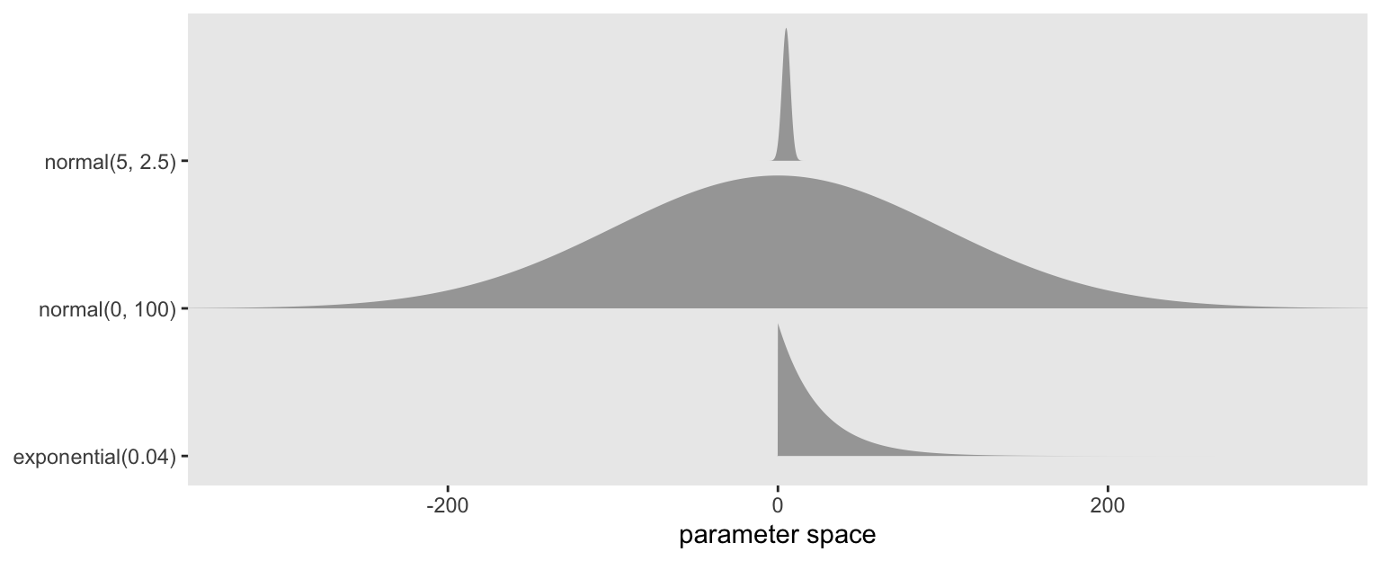
$$ \begin{align} \text{weight}_i & \sim \operatorname{Normal}(\mu_i, \sigma) \\ \mu_i & = \beta_0 + \beta_1 \text{height}_i \\ \beta_0 & \sim \operatorname{Normal}(0, 100) \\ \beta_1 & \sim \operatorname{Normal}(5, 2.5) \\ \sigma & \sim \operatorname{Exponential}(0.04), \end{align} $$

where weight values vary across \(i\) people, and they are modeled as normally distributed with a conditional mean \(\mu_i\) and [residual] standard deviation \(\sigma\). The conditional mean is defined by an intercept \(\beta_0\) and slope \(\beta_1\) for the predictor variable height. This time we discuss the priors in reverse order.

The \(\sigma\) parameter has changed meaning from a unconditional standard deviation to a conditional or residual standard deviation. Before we used an exponential prior centered at 25 (cf. McElreath, 2020), and for simplicity here we do the same. Recall that the mean of the exponential distribution is the reciprocal of its single parameter \(\lambda\), and we therefore set \(\lambda = 1/25 = 0.04\).

Our new \(\beta_1\) parameter is the expected change in weight for a one-unit change¹ in the predictor height. Given a normal prior, the values of a mean of five and standard deviation of 2.5 may seem oddly specific. A few things: My experience as a human living in the world among other humans tells me the \(\beta_1\) parameter will be positive, so a good theory-informed priors should down rate negative values. When I did a quick web search on the relation between height and weight, Peterson et al. ( 2016) popped up which indicated that given the typical adult range for height, a one inch increase predicts about a 5 lb increase in ideal weight. By scaling the prior with 2.5, that puts about 95% of the prior probability between zero and twice that value.

In this model, I think \(\beta_0\) is the most challenging parameter for which to set a prior. The intercept, recall, is the expected value when the predictor variable is set to zero. At a first stab, you might insist that a hypothetical person zero inches tall would have to also weight zero pounds. But bear in mind we are fitting a simple linear model, which has no simple way to enforce such a constraint. For that we’d probably want some kind of exciting non-linear model.² Also, given that we are using weight in inches, and given these data were simulated to resemble typical US adults, none of the weight values are remotely close to zero, which means that not only we, but the model itself will have a very difficult time estimating the expected value at zero. So to express this uncertainty, but to still suggest our best guess is the value will be around zero, we use a normal prior centered at zero, with a large scale of 100.

Here’s a quick look at the priors.

c(prior(normal(0, 100), class = b, coef = Intercept),
  prior(normal(5, 2.5), class = b),
  prior(exponential(0.04), class = sigma)) |> 
  parse_dist() |> 

  ggplot(aes(y = prior)) +
  stat_slab(aes(dist = .dist_obj),
            n = 5001, normalize = "xy", p_limits = c(0.0001, 0.9999)) +
  scale_y_discrete(NULL, expand = expansion(mult = 0.1)) +
  xlab("parameter space") +
  coord_cartesian(xlim = c(-325, 325)) +
  theme(panel.grid = element_blank())

Center the predictor

Some of my more experienced readers might wonder why I haven’t made things easier on myself by centering the predictor variable. Then we could drop that annoyingly wide \(\operatorname{Normal}(0, 100)\) prior for \(\beta_0\). Yes, that’s a great strategy in many contexts. Mean centering predictor variables is a big deal with brms, particularly with how you set your priors.³ It’s such a big deal that it will be the focus of the next post. But the mean-centering issue and how it relates to brms syntax complicates the underlying Stan code in ways I think would be prohibitively confusing at this point. The Stan code is simpler for a model fit with a non-standardized predictor. And plus, it’s nice to learn how to fit a Stan model with a non-centered predictor. As an applied researcher, I like it when I have options.

brms workflow

For brms users who’ve read the first post in this series, there should be few surprises here.

Fit the model with brm()

We can fit this model with brms like so.

brm2 <- brm(
  data = d,
  family = gaussian,
  bf(weight ~ 1 + height, center = FALSE),
  prior = prior(normal(0, 100), class = b, coef = Intercept) +
    prior(normal(5, 2.5), class = b) +
    prior(exponential(0.04), class = sigma),
  cores = 4, seed = 1,
  file = "fits/brm2")

The only noteworthy part of the model code is how we wrapped our formula line in the bf() function, in which we also set center = FALSE. Those details have to do with setting the prior for \(\beta_0\) using the current version of height that is not mean centered. You can execute ?brmsformula in your console for the technical documentation. We’ll have more to say on that whole issue in the next post. For now, just go with it.

Check the parameter summary.

print(brm2)

##  Family: gaussian 
##   Links: mu = identity; sigma = identity 
## Formula: weight ~ 1 + height 
##    Data: d (Number of observations: 100) 
##   Draws: 4 chains, each with iter = 2000; warmup = 1000; thin = 1;
##          total post-warmup draws = 4000
## 
## Regression Coefficients:
##           Estimate Est.Error l-95% CI u-95% CI Rhat Bulk_ESS Tail_ESS
## Intercept   -67.99     39.23  -145.66     9.58 1.01     1178     1327
## height        3.39      0.59     2.24     4.56 1.01     1172     1343
## 
## Further Distributional Parameters:
##       Estimate Est.Error l-95% CI u-95% CI Rhat Bulk_ESS Tail_ESS
## sigma    28.87      2.06    25.01    33.31 1.00     1719     1431
## 
## Draws were sampled using sampling(NUTS). For each parameter, Bulk_ESS
## and Tail_ESS are effective sample size measures, and Rhat is the potential
## scale reduction factor on split chains (at convergence, Rhat = 1).

We might use the posterior draws to plot the fitted line against the data. To better understand the role of the intercept \(\beta_0\), we will extend the regression line well past the lower limit of the data all the way to zero. For kicks and giggles, we’ll also superimpose the OLS regression line in red.

xmax <- max(d$height) |> ceiling()

data.frame(height = 0:xmax) |> 
  add_epred_draws(brm2) |> 
  rename(weight = .epred) |> 
  
  ggplot(aes(x = height, y = weight)) +
  stat_lineribbon(.width = 0.95,
                  color = "steelblue4", fill = "steelblue1", linewidth = 1/2) +
  geom_point(data = d) +
  stat_smooth(data = d,
              formula = 'y ~ x', method = "lm", se = FALSE,
              color = "red") +
  theme(panel.grid = element_blank())

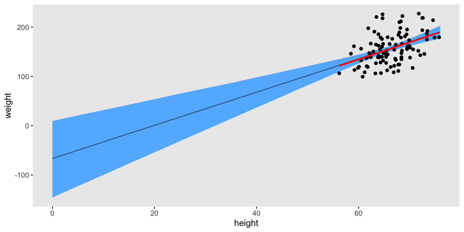
In this case, our Bayesian regression line matched nicely with the OLS line.⁴ But also, hopefully it now makes sense why we used such a weak prior for \(\beta_0\). The observed data are long ways from zero, and there’s no good way to enforce an exact-zero intercept with a simple linear model.⁵

Extract the Stan code with stancode()

As we learned in the first post, we can extract the Stan code underlying our brm2 model with the stancode() function.

stancode(brm2)

## // generated with brms 2.22.0
## functions {
## }
## data {
##   int<lower=1> N;  // total number of observations
##   vector[N] Y;  // response variable
##   int<lower=1> K;  // number of population-level effects
##   matrix[N, K] X;  // population-level design matrix
##   int prior_only;  // should the likelihood be ignored?
## }
## transformed data {
## }
## parameters {
##   vector[K] b;  // regression coefficients
##   real<lower=0> sigma;  // dispersion parameter
## }
## transformed parameters {
##   real lprior = 0;  // prior contributions to the log posterior
##   lprior += normal_lpdf(b[1] | 0, 100);
##   lprior += normal_lpdf(b[2] | 5, 2.5);
##   lprior += exponential_lpdf(sigma | 0.04);
## }
## model {
##   // likelihood including constants
##   if (!prior_only) {
##     target += normal_id_glm_lpdf(Y | X, 0, b, sigma);
##   }
##   // priors including constants
##   target += lprior;
## }
## generated quantities {
## }

Many of the features in this Stan code mirror those from the Stan code from the first post. But if you look closely, there are some new features in the data, parameters and model blocks, and now the transformed data and generated quantities blocks are empty! We will discuss those new features in the sections below.

Extract the Stan data with standata()

Investigate the data brms actually passed onto Stan with the standata() function.

standata(brm2) |> 
  str()

## List of 5
##  $ N         : int 100
##  $ Y         : num [1:100(1d)] 142 210 162 138 194 ...
##  $ K         : int 2
##  $ X         : num [1:100, 1:2] 1 1 1 1 1 1 1 1 1 1 ...
##   ..- attr(*, "dimnames")=List of 2
##   .. ..$ : chr [1:100] "1" "2" "3" "4" ...
##   .. ..$ : chr [1:2] "Intercept" "height"
##   ..- attr(*, "assign")= int [1:2] 0 1
##  $ prior_only: int 0
##  - attr(*, "class")= chr [1:2] "standata" "list"

This is largely the same as in the last post. In the sections below, we will learn about the mysterious X and K elements.

rstan workflow

We will fit four rstan versions of the brm2 model. We start simple with the first model stan2.1. We then take a whirlwind review of the major Stan-code insights from the last post with stan2.2. With stan2.3 we learn about model matrices and parameter vectors, and with stan2.4 we meet a new family of functions parameterized for the generalized linear model.

stan2.1, start simple

As a first step, we make a data list with the compose_data() function.

stan_data <- d |> 
  select(weight, height) |> 
  compose_data()

str(stan_data)

## List of 3
##  $ weight: num [1:100(1d)] 142 210 162 138 194 ...
##  $ height: num [1:100(1d)] 63.9 68 63.9 70.1 72.5 64.2 61.9 62.1 74.9 63.5 ...
##  $ n     : int 100

The weight and height columns have been saved as named numeric vectors in the list, and compose_data() automatically added the n scalar value defining the number of cases in the data. We don’t have analogues to the X and K elements yet, but those will come later.

As in the last post, our first stan() model will use a simplified version of Bürkner’s Stan code. You might compare this with the first example in the Regression Models chapter of the Stan User’s Guide ( Stan Development Team, 2024c).

model_code_2.1 <- '
data {
  int<lower=1> n;    // Total number of observations
  vector[n] weight;  // Response variable
  vector[n] height;  // Predictor variable
}
parameters {
  real beta0;           // Intercept
  real beta1;           // Slope
  real<lower=0> sigma;  // Dispersion parameter
}
model {
  weight ~ normal(beta0 + beta1 * height, sigma);  // Likelihood
  beta0 ~ normal(0, 100);                          // Priors
  beta1 ~ normal(5, 2.5);
  sigma ~ exponential(0.04);
}
'

In the data block we have added a line for the predictor variable height, which is a vector of length n. In the parameters block we now have an intercept and a slope, which we’ve defined on separate lines. We did not have to choose the names beta0 and beta1, and you are at liberty to alter them if you’re following along on your own computer. Notice we’re using the distribution syntax for the likelihood and priors in the model block. We’ll switch that out for more sophisticated syntax in the models to come. In the likelihood line, notice how we’re defining the entire linear model right there in the first parameter of normal(). There are other ways to do this, and we’ll explore those below. But for now, notice how we used the syntax of beta1 * height, where we multiply the beta1 slope with the height vector using the * operator. This is more explicit than the typical 1 + height syntax we use in R functions like brm() or lm(). At this point, I’m hoping the syntax we used for the priors will make sense.

We’re ready to fit the model with stan().

stan2.1 <- stan(
  data = stan_data,
  model_code = model_code_2.1,
  cores = 4, seed = 1)

The print() summary for our stan() model is very similar to the output for brm2 above, but it’s not identical. By the end of this post, we will perfectly match the draws from brm2.

# summary(brm2)
print(stan2.1, probs = c(0.025, 0.975))

## Inference for Stan model: anon_model.
## 4 chains, each with iter=2000; warmup=1000; thin=1; 
## post-warmup draws per chain=1000, total post-warmup draws=4000.
## 
##          mean se_mean    sd    2.5%   97.5% n_eff Rhat
## beta0  -66.78    1.30 42.06 -150.99   15.81  1047    1
## beta1    3.37    0.02  0.63    2.12    4.64  1047    1
## sigma   28.97    0.05  2.09   25.23   33.33  1715    1
## lp__  -384.67    0.04  1.24 -387.94 -383.25  1113    1
## 
## Samples were drawn using NUTS(diag_e) at Sun Jul 13 17:17:18 2025.
## For each parameter, n_eff is a crude measure of effective sample size,
## and Rhat is the potential scale reduction factor on split chains (at 
## convergence, Rhat=1).

stan2.2 and a quick Stan code review

We’ll use this section to review all the Stan syntax insights we learned in the first post, and then add them to the model in quick succession.

lprior and target += normal_lpdf

Our first step is to define the lprior vector in the transformed parameters block. We also switch to the log probability density function syntax for the likelihood and priors, with its exciting looking += operator. In short, the lprior is the log of the prior density, and target is a reserved term used for the log of the posterior density. For more details on these additions, go back and review this section from the first post.

data {
  int<lower=1> n;
  vector[n] weight;
  vector[n] height;
}
parameters {
  real beta0;
  real beta1;
  real<lower=0> sigma;
}
transformed parameters {
  real lprior = 0;  // Prior contributions to the log posterior
  lprior += normal_lpdf(beta0 | 0, 100);
  lprior += normal_lpdf(beta1 | 5, 2.5);
  lprior += exponential_lpdf(sigma | 0.04);
}
model {
  target += normal_lpdf(weight | beta0 + beta1 * height, sigma);  // Likelihood
  target += lprior;                                               // Priors
}

You can fit a model using this model_code as an intermediate step, but I’m going to press forward.

prior_only and if

Next we can add that if statement to the model block that can handle the prior_only option (Should we sample from the posterior, or from the prior?). For more details on these additions, go back and review this section from the first post.

data {
  int<lower=1> n;
  vector[n] weight;
  vector[n] height;
  int prior_only;  // Should the likelihood be ignored?
}
parameters {
  real beta0;
  real beta1;
  real<lower=0> sigma;
}
transformed parameters {
  real lprior = 0;
  lprior += normal_lpdf(beta0 | 0, 100);
  lprior += normal_lpdf(beta1 | 5, 2.5);
  lprior += exponential_lpdf(sigma | 0.04);
}
model {
  // Likelihood
  if (!prior_only) {
    target += normal_lpdf(weight | beta0 + beta1 * height, sigma);
  }
  // Priors
  target += lprior;
}

For this step, we need to add that prior_only scalar to the data list, which we do like so.

stan_data <- d |> 
  select(weight, height) |> 
  compose_data(prior_only = as.integer(FALSE))

str(stan_data)

## List of 4
##  $ weight    : num [1:100(1d)] 142 210 162 138 194 ...
##  $ height    : num [1:100(1d)] 63.9 68 63.9 70.1 72.5 64.2 61.9 62.1 74.9 63.5 ...
##  $ n         : int 100
##  $ prior_only: int 0

You can fit a model using this model_code as an intermediate step, but I’m going to press forward, still. We have one more point to review, and this time that review should relieve an unresolved tension from the first post. Get excited!

mu += Intercept, but better

You might recall that back in the first post ( here), we discussed this mu += Intercept line Bürkner smuggled into the middle of his model block. It didn’t make any sense in the context of an intercept-only model, but we followed along anyway and let the tension build. Take another look at the current state of our likelihood line.

target += normal_lpdf(weight | beta0 + beta1 * height, sigma);

The linear function in the model is starting to take up a lot of horizontal space, and you could only imagine how this might spiral out of control if we were to add more predictor terms to the model. So one nice trick is to define a new term mu, and then just substitute that term into the normal_lpdf() function.

vector[n] mu = rep_vector(0.0, n);
mu += beta0 + beta1 * height;
target += normal_lpdf(weight | mu, sigma);

Notice how before we define mu with the linear model, we first declare its dimensions in the opening line vector[n] mu = rep_vector(0.0, n). When we use code like this within a model block, the posterior will not return samples from mu. It will just return draws from the beta0 and beta1 parameters instead. But if we did want to sample from mu as well, we could define it in the transformed parameters or generated quantities blocks.

For our use case, here’s what this looks like in full.

model_code_2.2 <- '
data {
  int<lower=1> n;
  vector[n] weight;
  vector[n] height;
  int prior_only;
}
parameters {
  real beta0;
  real beta1;
  real<lower=0> sigma;
}
transformed parameters {
  real lprior = 0;
  lprior += normal_lpdf(beta0 | 0, 100);
  lprior += normal_lpdf(beta1 | 5, 2.5);
  lprior += exponential_lpdf(sigma | 0.04);
}
model {
  // Likelihood
  if (!prior_only) {
    // Initialize linear predictor term
    vector[n] mu = rep_vector(0.0, n);
    mu += beta0 + beta1 * height;
    target += normal_lpdf(weight | mu, sigma);
  }
  // Priors
  target += lprior;
}
'

Now the line for the likelihood, target += normal_lpdf(weight | mu, sigma), no longer takes up all that horizontal space. And hopefully now you can also make sense of Bürkner’s comment: Initialize linear predictor term. mu is the linear predictor term. Time to fit the model with stan().

stan2.2 <- stan(
  data = stan_data,
  model_code = model_code_2.2,
  cores = 4, seed = 1)

The only major change in the print() output is the addition of the lprior line. Again, notice how there is no line for mu. Because we only defined mu in the model block, it was just temporary.

# summary(brm2)
# print(stan2.1, probs = c(0.025, 0.975))
print(stan2.2, probs = c(0.025, 0.975))

## Inference for Stan model: anon_model.
## 4 chains, each with iter=2000; warmup=1000; thin=1; 
## post-warmup draws per chain=1000, total post-warmup draws=4000.
## 
##           mean se_mean    sd    2.5%   97.5% n_eff Rhat
## beta0   -64.42    1.33 41.90 -144.28   18.55   987    1
## beta1     3.33    0.02  0.63    2.09    4.54   987    1
## sigma    28.94    0.05  2.07   25.20   33.29  1711    1
## lprior  -12.29    0.01  0.21  -12.82  -12.03  1051    1
## lp__   -487.14    0.03  1.21 -490.18 -485.74  1302    1
## 
## Samples were drawn using NUTS(diag_e) at Sun Jul 13 17:18:16 2025.
## For each parameter, n_eff is a crude measure of effective sample size,
## and Rhat is the potential scale reduction factor on split chains (at 
## convergence, Rhat=1).

stan2.3 with model.matrix()

It’s time to learn some new Stan syntax tricks. Before we do, we’ll want to discuss some statistical notation.

Compact notation and design matrices

When I express my models in statistical notation, I prefer the style

$$ \mu_i = \beta_0 + \beta_1 x_i $$

for models with a single predictor \(x\). When I have multiple predictors, I just generalize to

$$ \mu_i = \beta_0 + \beta_1 x_{1i} + \dots + \beta_K x_{Ki}, $$

where \(k\) is a predictor index and \(K\) is the total number of predictor variables. I find this notation style simple and easy to read, and of all the ways to write a linear model, this is the one I suspect will be the most accessible to my substantive colleagues.⁶ However, this style of equation doesn’t work well when \(K\) increases beyond the middle single-digit range.

One solution is the notation of

$$ \mu_i = \alpha + \sum_{k = 1}^K \beta_k x_{ki}, $$

where we now refer to the intercept as \(\alpha\), and we use the summation operator \(\sum(\cdot)\) as a shorthand for \(\beta_1 x_{1i} + \dots + \beta_K x_{Ki}\). We can use an even more compact notation of

$$ \mathbf m = \mathbf{Xb}. $$

This is matrix notation, for which \(\mathbf m\) is a vector of predicted means which is the same length as the sample data (100 rows in our case). The \(\mathbf X\) term is a matrix of predictor values, which includes one column for each of the predictor variables and an initial column that is a vector of 1’s for the intercept. The \(\mathbf b\) term is a vector of parameters, which begins with the intercept and ends with the final predictor \(x_K\). We could try to write this out more explicitly as something like

$$\begin{bmatrix} \mu_1 \\ \mu_2 \\ \vdots \\ \mu_N \end{bmatrix} = \begin{bmatrix} 1 & x_{11} & \dots & x_{K1} \\ 1 & x_{12} & \dots & x_{K2} \\ \vdots & \vdots & \ddots & \vdots \\ 1 & x_{1N} & \dots & x_{KN} \end{bmatrix} \begin{bmatrix} \beta_0 \\ \beta_1 \\ \vdots \\ \beta_K \end{bmatrix}.$$

Data matrices and parameter vectors in Stan

In R, we can define a model matrix with the model.matrix() function.⁷ For our model, that can look like so.

# Define a model matrix
mm_2.3 <- model.matrix(data = d, object = ~height)

# What?
str(mm_2.3)

##  num [1:100, 1:2] 1 1 1 1 1 1 1 1 1 1 ...
##  - attr(*, "dimnames")=List of 2
##   ..$ : chr [1:100] "1" "2" "3" "4" ...
##   ..$ : chr [1:2] "(Intercept)" "height"
##  - attr(*, "assign")= int [1:2] 0 1

head(mm_2.3)

##   (Intercept) height
## 1           1   63.9
## 2           1   68.0
## 3           1   63.9
## 4           1   70.1
## 5           1   72.5
## 6           1   64.2

The mm_2.3 object has two vectors: The first vector is a sequence of 1’s for the intercept, and the second vector has the values for the predictor height. In the notation above, these would be

$$\begin{bmatrix} 1 & x_{11} \\ 1 & x_{12} \\ \vdots & \vdots \\ 1 & x_{1N} \end{bmatrix},$$

where \(x_1\) is height, and \(N\) is our scalar value n. We can use this mm_2.3 object to define two new elements with the compose_data() function. The first will be X, to stand for the entire model matrix mm_2.3. The second will be k, the number of columns (i.e., “predictors”) in the design matrix.

stan_data <- d |> 
  select(weight) |> 
  compose_data(k = ncol(mm_2.3),
               X = mm_2.3,
               prior_only = as.integer(FALSE))

str(stan_data)

## List of 5
##  $ weight    : num [1:100(1d)] 142 210 162 138 194 ...
##  $ n         : int 100
##  $ k         : int 2
##  $ X         : num [1:100, 1:2] 1 1 1 1 1 1 1 1 1 1 ...
##   ..- attr(*, "dimnames")=List of 2
##   .. ..$ : chr [1:100] "1" "2" "3" "4" ...
##   .. ..$ : chr [1:2] "(Intercept)" "height"
##   ..- attr(*, "assign")= int [1:2] 0 1
##  $ prior_only: int 0

It’s important to notice that up until this point we’ve only been referring to variables like \(x_1\) (height) as predictors. But with this kind of model matrix, we are also including the vector of 1’s for the intercept as a “predictor.” Thus in that sense, our model matrix has k == 2 predictors.

Notice how because we have added our height values to the data list within the X model matrix, we no longer add them in from the data frame d. That is, we now just use d |> select(weight) in the opening lines of the code.

We can add this information to the data block of our model_code like so.⁸

model_code_2.3 <- '
data {
  int<lower=1> n;
  int<lower=1> k;  // Number of beta coefficients in the linear model
  vector[n] weight;
  matrix[n, k] X;  // Design matrix for the beta coefficients
  int prior_only;
}
parameters {
  vector[k] b;  // Regression coefficients (beta coefficients)
  real<lower=0> sigma;
}
transformed parameters {
  real lprior = 0;
  lprior += normal_lpdf(b[1] | 0, 100);
  lprior += normal_lpdf(b[2] | 5, 2.5);
  lprior += exponential_lpdf(sigma | 0.04);
}
model {
  if (!prior_only) {
    // Linear model defined in matrix algebra notation Xb
    target += normal_lpdf(weight | X * b, sigma);
  }
  target += lprior;
}
'

We have several points of interest. Focus on the data block, first.

data {
  int<lower=1> n;
  int<lower=1> k;  // Number of beta coefficients in the linear model
  vector[n] weight;
  matrix[n, k] X;  // Design matrix for the beta coefficients
  int prior_only;
}

We have declared our k scalar in the second line. We no longer declare the height values as a vector, like we did in earlier models. But now instead we declare the design matrix X as a matrix of n rows and k columns.

Next focus on the parameters block.

parameters {
  vector[k] b;  // Regression coefficients (beta coefficients)
  real<lower=0> sigma;
}

We have dropped those two lines that used to declare beta0 and beta1. Now we instead have a vector of b coefficients of length k, which is the first time we’ve seen a vector of parameters in this blog series. This is the code instantiation of what we might have described in statistical notation above as

$$\begin{bmatrix} \beta_0 \\ \beta_1 \end{bmatrix}.$$

As there’s nothing new for us in the transformed parameters block, we finally focus instead on the model block.

model {
  if (!prior_only) {
    // Linear model defined in matrix algebra notation Xb
    target += normal_lpdf(weight | X * b, sigma);
  }
  target += lprior;
}

Exciting as it was in the last section, we have dropped all that mu += beta0 + beta1 * height stuff. Now we instead define the entire linear model with the compact syntax of X * b, which you might notice looks a lot like the matrix algebra notation \(\mathbf{Xb}\) we just learned about in the equations above. That is, we have specified the linear model

$$\mathbf{Xb} = \begin{bmatrix} 1 & x_{1,1} \\ 1 & x_{1,2} \\ \vdots & \vdots \\ 1 & x_{1,100} \end{bmatrix} \begin{bmatrix} \beta_0 \\ \beta_1 \end{bmatrix}.$$

We’re ready to fit the model with stan().

stan2.3 <- stan(
  data = stan_data,
  model_code = model_code_2.3,
  cores = 4, seed = 1)

Check the summary.

# summary(brm2)
# print(stan2.1, probs = c(0.025, 0.975))
# print(stan2.2, probs = c(0.025, 0.975))
print(stan2.3, probs = c(0.025, 0.975))

## Inference for Stan model: anon_model.
## 4 chains, each with iter=2000; warmup=1000; thin=1; 
## post-warmup draws per chain=1000, total post-warmup draws=4000.
## 
##           mean se_mean    sd    2.5%   97.5% n_eff Rhat
## b[1]    -65.51    1.34 41.11 -147.07   17.45   944    1
## b[2]      3.35    0.02  0.62    2.10    4.57   936    1
## sigma    28.91    0.05  1.98   25.44   33.04  1502    1
## lprior  -12.28    0.01  0.22  -12.86  -12.03  1037    1
## lp__   -487.06    0.04  1.22 -490.27 -485.70  1169    1
## 
## Samples were drawn using NUTS(diag_e) at Sun Jul 13 17:19:17 2025.
## For each parameter, n_eff is a crude measure of effective sample size,
## and Rhat is the potential scale reduction factor on split chains (at 
## convergence, Rhat=1).

Overall, the parameter summaries are very similar to those from stan2.2. But notice the names of the first two rows. When we use this approach, all \(\beta\) coefficients in the model now take generic names b[k], ranging from \(1, \dots, K\). Even though we⁹ often refer to the intercept as \(\beta_0\), and so on, here the intercept is b[1]. To the best of my knowledge, there is no simple way to fix this when using this approach to fitting models with Stan. The first index in a vector is a 1, not a zero. We won’t have a good solution to that challenge in this post, but we will present an alternative in the third post. For now, let’s prepare for one last Stan syntax trick.

stan2.4 with the normal_id_glm_lpdf() function

Here’s the final version of the model_code for this post.

model_code_2.4 <- '
data {
  int<lower=1> n;
  int<lower=1> k;
  vector[n] weight;
  matrix[n, k] X;
  int prior_only;
}
parameters {
  vector[k] b;
  real<lower=0> sigma;
}
transformed parameters {
  real lprior = 0;
  lprior += normal_lpdf(b[1] | 0, 100);
  lprior += normal_lpdf(b[2] | 5, 2.5);
  lprior += exponential_lpdf(sigma | 0.04);
}
model {
  if (!prior_only) {
    target += normal_id_glm_lpdf(weight | X, 0, b, sigma);
  }
  target += lprior;
}
'

The only new line is for the likelihood in the model block. Following the syntax in Bürkner’s Stan code, we have abandoned the normal_lpdf() function for normal_id_glm_lpdf(). Stan provides a family of functions parameterized for the generalized linear model. This family of functions follows the naming convention of distribution_link_glm_function(). In this case, we are using the Gaussian distribution (normal), the identity link (id), and the log probability density function (lpdf). For the documentation, go here for the relevant section of the Stan Functions Reference ( Stan Development Team, 2024b). On the left side of the | bar, we input the response variable weight. The four arguments on the right side of the | bar are \(x, \alpha, \beta, \sigma\). For the first of those four, we input our model matrix X, which includes a constant vector of 1 for the intercept and a vector of the numeric values of the predictor height. In our case, we are not using the \(\alpha\) argument because we have included the intercept in X. In the next post, however, we will see an example of how we can use \(\alpha\). But notice we do input our vector of b parameters in the \(\beta\) argument. Perhaps not surprisingly at this point, we input our sigma parameter in the final argument \(\sigma\). In the Stan Functions Reference, we read this function is designed to provide “a more efficient implementation of linear regression than a manually written regression in terms of a normal distribution and matrix multiplication.”

Let’s fit the model and see.

stan2.4 <- stan(
  data = stan_data,
  model_code = model_code_2.4,
  cores = 4, seed = 1)

Check the summary.

# summary(brm2)
# print(stan2.1, probs = c(0.025, 0.975))
# print(stan2.2, probs = c(0.025, 0.975))
# print(stan2.3, probs = c(0.025, 0.975))
print(stan2.4, probs = c(0.025, 0.975))

## Inference for Stan model: anon_model.
## 4 chains, each with iter=2000; warmup=1000; thin=1; 
## post-warmup draws per chain=1000, total post-warmup draws=4000.
## 
##           mean se_mean    sd    2.5%   97.5% n_eff Rhat
## b[1]    -67.99    1.15 39.23 -145.66    9.58  1168 1.01
## b[2]      3.39    0.02  0.59    2.24    4.56  1162 1.01
## sigma    28.87    0.05  2.06   25.01   33.31  1728 1.00
## lprior  -12.28    0.01  0.21  -12.83  -12.02  1118 1.01
## lp__   -487.07    0.03  1.18 -489.98 -485.72  1298 1.00
## 
## Samples were drawn using NUTS(diag_e) at Sun Jul 13 17:20:21 2025.
## For each parameter, n_eff is a crude measure of effective sample size,
## and Rhat is the potential scale reduction factor on split chains (at 
## convergence, Rhat=1).

Was the normal_id_glm_lpdf() method efficient in terms of speed relative to the normal_lpdf() method? We can extract the warmup and sample times with the get_elapsed_time() function.

get_elapsed_time(stan2.3)  # `normal_lpdf()` method

##         warmup sample
## chain:1  0.191  0.149
## chain:2  0.202  0.136
## chain:3  0.169  0.123
## chain:4  0.170  0.124

get_elapsed_time(stan2.4)  # `normal_id_glm_lpdf()` method

##         warmup sample
## chain:1  0.097  0.089
## chain:2  0.101  0.099
## chain:3  0.113  0.085
## chain:4  0.122  0.091

Yes, it turns out the normal_id_glm_lpdf() method was indeed more efficient for both stages, and across all four chains.

Speaking of comparison, it’s now time to show our stan()-based stan2.4 model contains identical results for the HMC draws as the brm() benchmark brm2. As a first step, we extract and save the posterior draws with as_draws_df().

draws_brm2    <- as_draws_df(brm2)
draws_stan2.4 <- as_draws_df(stan2.4)

# Check the structures of the objects
glimpse(draws_brm2)

## Rows: 4,000
## Columns: 8
## $ b_Intercept <dbl> -16.94807, -39.02279, -113.91742, -117.34356, -118.47045, …
## $ b_height    <dbl> 2.638817, 2.974173, 4.055828, 4.193456, 4.097895, 3.244547…
## $ sigma       <dbl> 27.57305, 27.82910, 31.42171, 31.84472, 31.56111, 31.90749…
## $ lprior      <dbl> -12.14151, -12.09583, -12.55526, -12.59252, -12.60752, -12…
## $ lp__        <dbl> -486.5733, -486.0265, -487.2386, -488.3593, -487.8438, -48…
## $ .chain      <int> 1, 1, 1, 1, 1, 1, 1, 1, 1, 1, 1, 1, 1, 1, 1, 1, 1, 1, 1, 1…
## $ .iteration  <int> 1, 2, 3, 4, 5, 6, 7, 8, 9, 10, 11, 12, 13, 14, 15, 16, 17,…
## $ .draw       <int> 1, 2, 3, 4, 5, 6, 7, 8, 9, 10, 11, 12, 13, 14, 15, 16, 17,…

glimpse(draws_stan2.4)

## Rows: 4,000
## Columns: 8
## $ `b[1]`     <dbl> -16.94807, -39.02279, -113.91742, -117.34356, -118.47045, -…
## $ `b[2]`     <dbl> 2.638817, 2.974173, 4.055828, 4.193456, 4.097895, 3.244547,…
## $ sigma      <dbl> 27.57305, 27.82910, 31.42171, 31.84472, 31.56111, 31.90749,…
## $ lprior     <dbl> -12.14151, -12.09583, -12.55526, -12.59252, -12.60752, -12.…
## $ lp__       <dbl> -486.5733, -486.0265, -487.2386, -488.3593, -487.8438, -487…
## $ .chain     <int> 1, 1, 1, 1, 1, 1, 1, 1, 1, 1, 1, 1, 1, 1, 1, 1, 1, 1, 1, 1,…
## $ .iteration <int> 1, 2, 3, 4, 5, 6, 7, 8, 9, 10, 11, 12, 13, 14, 15, 16, 17, …
## $ .draw      <int> 1, 2, 3, 4, 5, 6, 7, 8, 9, 10, 11, 12, 13, 14, 15, 16, 17, …

Before we compare the two, we’ll need to rename two of the columns in draws_stan2.4.

draws_stan2.4 <- draws_stan2.4 |> 
  rename(b_Intercept = `b[1]`,
         b_height = `b[2]`)

Now that the two draws objects have the same column names, we can compare them directly with all.equal().

all.equal(draws_brm2, draws_stan2.4)

## [1] TRUE

Yes, their posterior draws are exactly the same. Success!

Wrap up

In this post we fit a single-level Gaussian model with a single continuous predictor with brms, and then fit the equivalent model with rstan. To replicate the brms results exactly, we expanded our Stan syntax skills to use model matrices, parameter vectors, and the normal_id_glm_lpdf() function for the likelihood. In the next post we grapple with how brms mean-centers predictors, and what that means for setting priors and for the underlying Stan code.

Happy coding, friends!

Thank the reviewers

I’d like to publicly acknowledge and thank

• Riccardo Fusaroli and
• Stephen J. Wild

for their kind efforts reviewing the draft of this post. Go team!

Do note the final editorial decisions were my own, and I do not think it would be reasonable to assume my reviewers have given blanket endorsements of the current version of this post.

Session information

sessionInfo()

## R version 4.4.3 (2025-02-28)
## Platform: aarch64-apple-darwin20
## Running under: macOS Ventura 13.4
## 
## Matrix products: default
## BLAS:   /Library/Frameworks/R.framework/Versions/4.4-arm64/Resources/lib/libRblas.0.dylib 
## LAPACK: /Library/Frameworks/R.framework/Versions/4.4-arm64/Resources/lib/libRlapack.dylib;  LAPACK version 3.12.0
## 
## locale:
## [1] en_US.UTF-8/en_US.UTF-8/en_US.UTF-8/C/en_US.UTF-8/en_US.UTF-8
## 
## time zone: America/Chicago
## tzcode source: internal
## 
## attached base packages:
## [1] stats     graphics  grDevices utils     datasets  methods   base     
## 
## other attached packages:
##  [1] posterior_1.6.1     ggdist_3.3.2        tidybayes_3.0.7    
##  [4] rstan_2.32.7        StanHeaders_2.32.10 brms_2.22.0        
##  [7] Rcpp_1.0.14         lubridate_1.9.3     forcats_1.0.0      
## [10] stringr_1.5.1       dplyr_1.1.4         purrr_1.0.4        
## [13] readr_2.1.5         tidyr_1.3.1         tibble_3.3.0       
## [16] ggplot2_3.5.2       tidyverse_2.0.0    
## 
## loaded via a namespace (and not attached):
##  [1] tidyselect_1.2.1     svUnit_1.0.6         viridisLite_0.4.2   
##  [4] farver_2.1.2         loo_2.8.0            fastmap_1.1.1       
##  [7] TH.data_1.1-2        tensorA_0.36.2.1     blogdown_1.20       
## [10] digest_0.6.37        estimability_1.5.1   timechange_0.3.0    
## [13] lifecycle_1.0.4      survival_3.8-3       magrittr_2.0.3      
## [16] compiler_4.4.3       rlang_1.1.6          sass_0.4.9          
## [19] tools_4.4.3          yaml_2.3.8           knitr_1.49          
## [22] labeling_0.4.3       bridgesampling_1.1-2 pkgbuild_1.4.8      
## [25] curl_6.0.1           plyr_1.8.9           RColorBrewer_1.1-3  
## [28] multcomp_1.4-26      abind_1.4-8          withr_3.0.2         
## [31] grid_4.4.3           stats4_4.4.3         xtable_1.8-4        
## [34] colorspace_2.1-1     inline_0.3.21        emmeans_1.10.3      
## [37] scales_1.4.0         MASS_7.3-64          dichromat_2.0-0.1   
## [40] cli_3.6.5            mvtnorm_1.3-3        rmarkdown_2.29      
## [43] generics_0.1.4       RcppParallel_5.1.10  rstudioapi_0.16.0   
## [46] reshape2_1.4.4       tzdb_0.4.0           cachem_1.0.8        
## [49] splines_4.4.3        bayesplot_1.13.0     parallel_4.4.3      
## [52] matrixStats_1.5.0    vctrs_0.6.5          V8_4.4.2            
## [55] Matrix_1.7-2         sandwich_3.1-1       jsonlite_1.8.9      
## [58] bookdown_0.40        hms_1.1.3            arrayhelpers_1.1-0  
## [61] jquerylib_0.1.4      glue_1.8.0           codetools_0.2-20    
## [64] distributional_0.5.0 stringi_1.8.7        gtable_0.3.6        
## [67] QuickJSR_1.8.0       pillar_1.11.0        htmltools_0.5.8.1   
## [70] Brobdingnag_1.2-9    R6_2.6.1             evaluate_1.0.1      
## [73] lattice_0.22-6       backports_1.5.0      bslib_0.7.0         
## [76] rstantools_2.4.0     coda_0.19-4.1        gridExtra_2.3       
## [79] nlme_3.1-167         checkmate_2.3.2      mgcv_1.9-1          
## [82] xfun_0.49            zoo_1.8-12           pkgconfig_2.0.3

References

Bürkner, P.-C. (2017). brms: An R package for Bayesian multilevel models using Stan. Journal of Statistical Software, 80(1), 1–28. https://doi.org/10.18637/jss.v080.i01
Bürkner, P.-C. (2018). Advanced Bayesian multilevel modeling with the R package brms. The R Journal, 10(1), 395–411. https://doi.org/10.32614/RJ-2018-017
Bürkner, P.-C. (2022). brms: Bayesian regression models using ’Stan’. https://CRAN.R-project.org/package=brms
Bürkner, P.-C., Gabry, J., Kay, M., & Vehtari, A. (2022). posterior: Tools for working with posterior distributions. https://CRAN.R-project.org/package=posterior
Kay, M. (2021). ggdist: Visualizations of distributions and uncertainty [Manual]. https://CRAN.R-project.org/package=ggdist
Kay, M. (2023). tidybayes: Tidy data and ’geoms’ for Bayesian models. https://CRAN.R-project.org/package=tidybayes
McElreath, R. (2020). Statistical rethinking: A Bayesian course with examples in R and Stan (Second Edition). CRC Press. https://xcelab.net/rm/statistical-rethinking/
Peterson, C. M., Thomas, D. M., Blackburn, G. L., & Heymsfield, S. B. (2016). Universal equation for estimating ideal body weight and body weight at any BMI. The American Journal of Clinical Nutrition, 103(5), 1197–1203. https://doi.org/10.3945/ajcn.115.121178
R Core Team. (2025). R: A language and environment for statistical computing. R Foundation for Statistical Computing. https://www.R-project.org/
Stan Development Team. (2024a). RStan: The R interface to Stan. https://mc-stan.org/
Stan Development Team. (2024b). Stan functions reference, Version 2.35. https://mc-stan.org/docs/functions-reference/
Stan Development Team. (2024c). Stan user’s guide, Version 2.35. https://mc-stan.org/docs/stan-users-guide/
Wickham, H. (2022). tidyverse: Easily install and load the ’tidyverse’. https://CRAN.R-project.org/package=tidyverse
Wickham, H., Averick, M., Bryan, J., Chang, W., McGowan, L. D., François, R., Grolemund, G., Hayes, A., Henry, L., Hester, J., Kuhn, M., Pedersen, T. L., Miller, E., Bache, S. M., Müller, K., Ooms, J., Robinson, D., Seidel, D. P., Spinu, V., … Yutani, H. (2019). Welcome to the tidyverse. Journal of Open Source Software, 4(43), 1686. https://doi.org/10.21105/joss.01686
-
Keep in mind change here is only used descriptively. Maybe
heighthas a simple causal relation toweight, maybe not. ↩︎ -
You can find several non-linear strategies for these kinds of data in McElreath ( 2020). ↩︎
In more ways than one. ↩︎
I compare the Bayesian line to OLS not because OLS is the benchmark. It isn’t. But given how small the data cloud is in this plot, it’s hard to judge how well the line is describing the data, and one could easily wonder how strongly the
\(\beta\)priors are influencing the posterior. Yes, the line describes the data well. No, these particular priors aren’t pushing the posterior that far from the likelihood. ↩︎ -
I mean, sure, you could do so by dropping the
\(\beta_0\)term altogether, which would effectively constrain the intercept to zero. But (a) that would do a worse job describing the observed data, and (b) it would no longer be a simple liner model, which is our framework here. ↩︎ -
I’m a clinical psychologist, recall. My fellow clinical psychologists generally don’t care for equations, but if you’re going to force an equation on them, this is the style I’d recommend. ↩︎
Execute
?model.matrixfor the documentation. ↩︎ -
See also the Matrix notation and vectorization section in the Stan User’s Guide ( Stan Development Team, 2024c). ↩︎
Or at least me, Solomon, anyway. ↩︎
- Posted on:
- July 13, 2025
- Length:
- 31 minute read, 6603 words