Learn Stan with brms, Part I

Stan code can be hard

Though I’m an ardent brms user, I’ve been learning more about Stan for another project. One of the ways you can learn more about Stan is by reviewing the Stan code underlying your brms models. But I’m guessing that if you’ve ever tried that, you discovered Paul Bürkner’s Stan code can be challenging to read. The purpose of this post, and the next couple posts to come, is to help demystify the Stan code from a few simple brms models.

I make assumptions

For this series, you’ll want to be familiar with Bayesian single-level regression. We’ll be sticking with Gaussian models for this series. For Bayesian regression beginners, I recommend the texts by Gelman and colleagues ( 2020), Kruschke ( 2015), or McElreath ( 2015, 2020). However, if applied Bayesian statistics is new to you, this probably isn’t the right time to wade through this blog series.

All code will be in R ( R Core Team, 2025). Data wrangling and plotting will rely heavily on the tidyverse ( Wickham et al., 2019; Wickham, 2022) and ggdist ( Kay, 2021). Bayesian models will be fit with brms ( Bürkner, 2017, 2018, 2022) and rstan ( Stan Development Team, 2024a).¹ We will post process our models with help from packages such as posterior ( Bürkner et al., 2022) and tidybayes ( Kay, 2023).

For the rstan package, do check out their website at https://mc-stan.org/rstan/. But since rstan is mainly an R interface for Stan, readers of this blog series will want to bookmark the resources at the Stan website https://mc-stan.org/docs/. Specifically, the Stan Functions Reference ( Stan Development Team, 2024b), the Stan Reference Manual ( Stan Development Team, 2024c), and the Stan User’s Guide ( Stan Development Team, 2024d). For ongoing education and debugging insights, I also recommend setting up a profile on the Stan Forums at https://discourse.mc-stan.org/.

Load the primary R packages.

library(tidyverse)
library(brms)
library(rstan)
library(tidybayes)
library(ggdist)
library(posterior)

We need data

The data were made with a custom function, which you can learn about in the appendix.

load(file = "data/d.rda")

The data are \(N = 100\) cases of height and weight values, simulated based on US adult benchmarks from a few decades ago. The units are inches and pounds.

glimpse(d)

## Rows: 100
## Columns: 3
## $ male   <dbl> 0, 1, 0, 1, 1, 0, 0, 0, 1, 0, 0, 0, 0, 0, 0, 1, 0, 0, 1, 1, 0, …
## $ height <dbl> 63.9, 68.0, 63.9, 70.1, 72.5, 64.2, 61.9, 62.1, 74.9, 63.5, 63.…
## $ weight <dbl> 141.7, 210.1, 162.5, 138.2, 193.8, 155.3, 197.8, 147.4, 178.9, …

Here’s what they look like in a scatter plot.

d |> 
  ggplot(aes(x = height, y = weight)) +
  geom_point() +
  theme(panel.grid = element_blank())

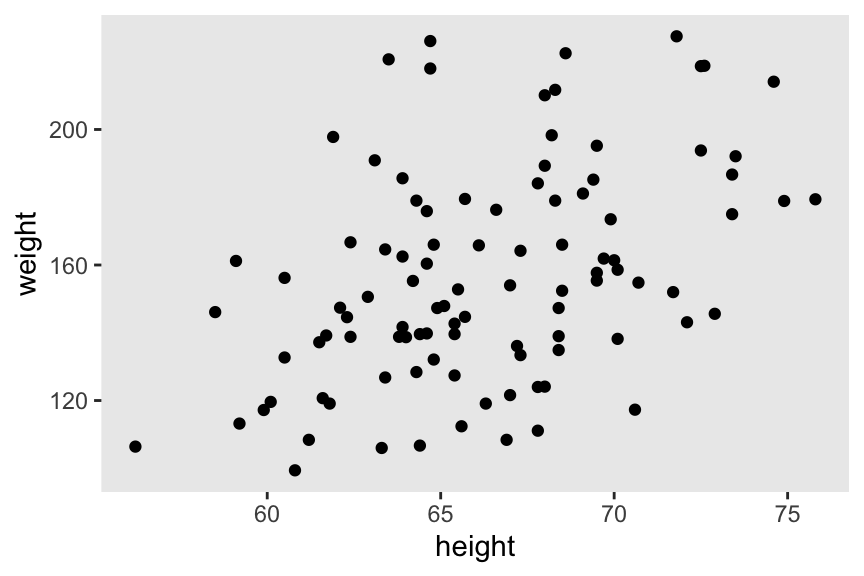
For this post and the next two to come, we will take weight as our response variable².

Focal model

To start this series off, we will fit the simple intercept-only model

\begin{align} \text{weight}_i & \sim \operatorname{Normal}(\mu, \sigma) \\ \mu & \sim \operatorname{Normal}(160, 25) \\ \sigma & \sim \operatorname{Exponential}(0.04), \end{align}

where weight values vary across \(i\) people, and they are modeled as normally distributed with a simple population mean \(\mu\) and standard deviation \(\sigma\). In terms more common among regression models, you could also write \(\mu = \beta_0\), the unconditional intercept. The last two rows are the priors, for which I’ll provide some detail next.

The data were simulated based on US adult norms from a few decades ago, and the cases are an even mixture of men and women. We like our heavy dinners and soft drinks here in the US, and so our average weight tends to be higher than other populations (e.g., Our World in Data, 2025). Based on self-reports from US adults from the early 1990s, their average weight at that time was around 160 pounds ( Saad, 2021), which is why I’ve centered the prior for \(\mu\) at 160. Setting the scale of the prior at 25 is a way to make it weak and uncertain on the scale of the data.

For the standard deviation of the weight distribution, I’m using the simple exponential prior, as recommended in McElreath ( 2020). The mean of the exponential distribution is the reciprocal of its single parameter \(\lambda\), and if we make a liberal guess the standard distribution is 25, that would mean \(\lambda = 1/25 = 0.04\).

You, of course, don’t have to use my priors. If you think they’re terrible, great! Set your own and see what happens as you follow along.³ You’ll probably learn more if you do.

brms workflow

I’m assuming readers of this series are already familiar with the brms basics. If you’re not, I’ve published several applied books on how to use brms, which you can find listed here. However, the last two subsections in this section may be new to even to intermediate brms users.

Fit the model with brm()

We can fit this model with brms like so.⁴

brm1 <- brm(
  data = d,
  family = gaussian,
  weight ~ 1,
  prior = prior(normal(160, 25), class = Intercept) +
    prior(exponential(0.04), class = sigma),
  cores = 4, seed = 1,
  file = "fits/brm1")

Check the parameter summary.

print(brm1)

##  Family: gaussian 
##   Links: mu = identity; sigma = identity 
## Formula: weight ~ 1 
##    Data: d (Number of observations: 100) 
##   Draws: 4 chains, each with iter = 2000; warmup = 1000; thin = 1;
##          total post-warmup draws = 4000
## 
## Regression Coefficients:
##           Estimate Est.Error l-95% CI u-95% CI Rhat Bulk_ESS Tail_ESS
## Intercept   156.67      3.12   150.51   162.55 1.00     3761     2729
## 
## Further Distributional Parameters:
##       Estimate Est.Error l-95% CI u-95% CI Rhat Bulk_ESS Tail_ESS
## sigma    32.07      2.28    28.09    36.95 1.00     3433     2425
## 
## Draws were sampled using sampling(NUTS). For each parameter, Bulk_ESS
## and Tail_ESS are effective sample size measures, and Rhat is the potential
## scale reduction factor on split chains (at convergence, Rhat = 1).

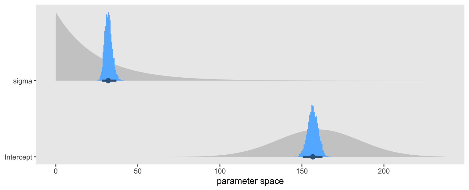
Our priors were a little high for \(\mu\), and a little low for \(\sigma\). But they were both well in the ballpark, so I’d call this a success. To get a better sense, here’s a plot of the parameter posteriors (blue) superimposed on their prior distributions (gray).

c(prior(normal(160, 25), class = Intercept),
  prior(exponential(0.04), class = sigma)) |> 
  parse_dist() |> 

  ggplot(aes(y = class)) +
  stat_slab(aes(dist = .dist_obj),
            fill = "gray80") +
  stat_histinterval(data = as_draws_df(brm1) |> 
                      pivot_longer(cols = sigma:Intercept, names_to = "class"),
                    aes(x = value),
                    .width = 0.95, color = "steelblue4", fill = "steelblue1") +
  scale_y_discrete(NULL, expand = expansion(mult = 0.1)) +
  xlab("parameter space") +
  theme(panel.grid = element_blank())

Extract the Stan code with stancode()

We can extract the Stan code underlying our brm() model with the stancode() function.

stancode(brm1)

## // generated with brms 2.22.0
## functions {
## }
## data {
##   int<lower=1> N;  // total number of observations
##   vector[N] Y;  // response variable
##   int prior_only;  // should the likelihood be ignored?
## }
## transformed data {
## }
## parameters {
##   real Intercept;  // temporary intercept for centered predictors
##   real<lower=0> sigma;  // dispersion parameter
## }
## transformed parameters {
##   real lprior = 0;  // prior contributions to the log posterior
##   lprior += normal_lpdf(Intercept | 160, 25);
##   lprior += exponential_lpdf(sigma | 0.04);
## }
## model {
##   // likelihood including constants
##   if (!prior_only) {
##     // initialize linear predictor term
##     vector[N] mu = rep_vector(0.0, N);
##     mu += Intercept;
##     target += normal_lpdf(Y | mu, sigma);
##   }
##   // priors including constants
##   target += lprior;
## }
## generated quantities {
##   // actual population-level intercept
##   real b_Intercept = Intercept;
## }

Even for a model without predictors, there’s a lot going on in that code. Fortunately, there are simpler ways to specify a model like this in Stan, and we’ll practice those first before building up to more sophisticated code like this. So if you’re intimidated already, great! This is the blog post for you.

Extract the Stan data with standata()

Though we usually use data frames to input our data to brms, Stan expects data in a different format. To see the data brms actually passed onto Stan, we can use the standata() function.

standata(brm1) |> 
  str()

## List of 6
##  $ N         : int 100
##  $ Y         : num [1:100(1d)] 142 210 162 138 194 ...
##  $ K         : int 1
##  $ Kc        : num 0
##  $ X         : num [1:100, 1] 1 1 1 1 1 1 1 1 1 1 ...
##   ..- attr(*, "dimnames")=List of 2
##   .. ..$ : chr [1:100] "1" "2" "3" "4" ...
##   .. ..$ : chr "Intercept"
##   ..- attr(*, "assign")= int 0
##  $ prior_only: int 0
##  - attr(*, "class")= chr [1:2] "standata" "list"

Surprised? We’ll explain the major features of that output below, and in the next two posts to come.

rstan workflow

In this section I’ll be pulling liberally from Kurz ( 2024), Chapter 1. Interested readers should go there for many more examples of Stan models fit to familiar data sets, especially if you like McElreath’s books.

We will be fitting six rstan versions of the brm1 model. We will start simple, and slowly build up our code until it matches all the major features from the stancode() output above. Though all of our rstan models will be similar to the one from brms, the sixth and final model will match it exactly. The remaining subsections are organized around the six models, and the first is a massive rstan introductory with subsections of its own.

stan1.1 and the rstan newbie bootcamp

Readers familiar with rstan might want to lightly browse through this section, and take whatever they may need. brms users new to rstan should probably work through it slowly, and spend some time with the resources cited within.

Stan likes data in lists

Many model-fitting functions in R allow for a variety of data types, including data frames, lists, free-floating vectors, and so on. Stan expects data in lists, and the primary model-fitting functions in the rstan package generally expect data lists, too. The tidybayes package includes a compose_data() function, which makes it easy to convert data frames into the list format we need. Here’s what this can look like for our use case.

stan_data <- d |> 
  select(weight) |> 
  compose_data()

# What?
str(stan_data)

## List of 2
##  $ weight: num [1:100(1d)] 142 210 162 138 194 ...
##  $ n     : int 100

The compose_data() function automatically added a scalar value n, which defines the number of rows in the original data frame. As we will see, scalar values defining various dimensions are important for the kind of syntax we use with rstan. There were several in the data from standata(brm1) above, but we only need n to start.

model_code and its blocks

Stan programs are organized into a series of program blocks, and those blocks are saved as a character string for the primary rstan functions.⁵ Following the schematic in the Program Blocks section in the Stan Reference Manual, those blocks are:

functions {
  // ... function declarations and definitions ...
}
data {
  // ... declarations ...
}
transformed data {
   // ... declarations ... statements ...
}
parameters {
   // ... declarations ...
}
transformed parameters {
   // ... declarations ... statements ...
}
model {
   // ... declarations ... statements ...
}
generated quantities {
   // ... declarations ... statements ...
}

These blocks must always be in this order, but not all Stan programs need all of the blocks. For example, our first version of the model only requires the data, parameters, and model blocks. Here’s what they look like, saved as a character string named model_code_1.1.

model_code_1.1 <- '
data {
  int<lower=1> n;    // Total number of observations
  vector[n] weight;  // Response variable
}
parameters {
  real mu;              // Unconditional mean (aka alpha, b_0, or beta_0)
  real<lower=0> sigma;  // Dispersion parameter
}
model {
  weight ~ normal(mu, sigma);  // Likelihood
  mu ~ normal(160, 25);        // Priors
  sigma ~ exponential(0.04);
}
'

In Stan program blocks, each line ends with a ;. As you can see in the model block, we can annotate the code with // marks. We’ll focus on each of the three program blocks in the subsections below.

Check the data block

Data declarations are a big deal with Stan. We’ll cover a few of the fine points in this section, but the primary information source is the Data Types and Declarations section of the Stan Reference Manual. At some time or another, you will want to study that material.

Here’s a focused look at our data block.

data {
  int<lower=1> n;    // Total number of observations
  vector[n] weight;  // Response variable
}

All the data required by the model must be declared in the data block. An important exception is if you define a transformed version of any of your data in the transformed data block, and we will see examples of that strategy later in the third post of this series. One generally defines one variable per line, but it is possible to declare multiple variables in a single line (see here).

It’s important to understand that Stan programs are read in order, top to bottom. Thus the first line in a data block often defines a scalar value we later use to define a data dimension. Recall how earlier we learned the compose_data() function automatically makes an n scalar, which defines the number of rows in the original data set. If you have more than one scalar value for your model, it’s generally a good idea to declare them all at the top.

With the syntax of int in this first line, we have declared that n scalar an integer. Stan can accept two primitive number types, which are int for integers and real for continuous numbers. There are other special types, such as complex, but I believe we will just be using int and real in this blog series.

Some values have constraints, and we have declared 1 to be the lowest integer value allowed for our n scalar by the <lower=1> syntax in our first line. Technically, we didn’t need to define this constraint for this example; the model will fit fine without it. In this case, the constraint will serve as a error check to make sure we have a least one case in our data. If you look back, you’ll see Bürkner also used this convention in his Stan code.

By the second line vector[n] weight, we have defined our weight response values as a vector of length n. Stan supports several data types, such as scalars, vectors, matrices, and arrays (see here). Though sequences of real values (such as weight) can be declared in vectors or arrays, sequences of integers go into arrays. If you try to declare a sequence of integer values as a vector, Stan will return an error. In my experience, properly juggling vectors and arrays has been a major source of frustration. Stan is picky, friends. Respect the data types.

Our parameters block

A good initial place to learn the technical details for the parameters block is in the Program block: parameters section of the Stan Reference Manual. Otherwise you can glean a lot of applied insights from the Regression Models section of the Stan User’s Guide.

Here’s a focused look at our parameters block.

parameters {
  real mu;              // Unconditional mean (aka alpha, b_0, or beta_0)
  real<lower=0> sigma;  // Dispersion parameter
}

Our unconditional mean parameter mu is declared as an unconstrained real value. Parameters can have constraints, and our syntax of real<lower=0> placed a lower boundary of zero for our \(\sigma\) parameter. It’s also possible to place upper boundaries, such as <lower=0, upper=1> for proportions. Though we don’t have any here, you can declare vectors and matrices of parameters too.

Our model block

In the above sections were we detailed our data and parameters blocks, all of their contents were what are called declarations. Whereas model blocks do allow for declarations, they also allow for statements. In short, declarations let you name data elements and model parameters, and statements tell Stan how the parameters should be computed. A great place to learn all about statements is the Statements section of the Stan Reference Manual. You might also read the brief Program block: model section of the Stan Reference Manual, or soak in all the applied examples in the Regression Models section of the Stan User’s Guide. When you’re really ready to get serious, you could browse though pretty much the whole of the Stan Functions Reference.

Here’s a focused look at our model block.

model {
  weight ~ normal(mu, sigma);  // Likelihood
  mu ~ normal(160, 25);        // Priors
  sigma ~ exponential(0.04);
}

My preference is to define the likelihood first, and then add the priors. I’ve seen many examples of the reverse, and sometimes they’re even shuffled all around. You pick whatever convention that makes sense for you and your collaborators, but I do recommend you choose a consistent format.

With the syntax of weight ~ normal(...) in our first line, we have defined the weight response variable as normally distributed, and as described with the two parameters named mu and sigma. Even though \(\mu\) and \(\sigma\) are the typical names for these parameters, we could have chosen different ones for the model. But had we wanted to do so, that would have required different code in the parameters block. For example, say we wanted to call our first parameter beta0 and our second parameter scale, we could have done this:

parameters {
  real beta0;
  real<lower=0> scale;
}
model {
  weight ~ normal(beta0, scale);
  beta0 ~ normal(160, 25);
  scale ~ exponential(0.04);
}

But anyways, this kind of likelihood syntax is often called the distribution syntax in Stan. It’s perhaps the most simple, and I generally like it the best. But there are many others, and Bürkner’s Stan code above uses an alternative we’ll discuss more below.

Notice that our prior lines follow a similar kind of syntax as our likelihood line for weight. Each prior line started with the parameter of interest on the left side, followed by the tilde ~, and then concluded with a distribution. Though not shown here, it is also possible to assign vectors of parameters to a common prior.

HMC sampling with stan()

To my eye, there are two basic ways to draw posterior samples from rstan. The simplest way is with stan(), and a handy alternative is to use the combo of stan_model() and sampling(). In this blog series we’ll just practice with the stan() function. The two main arguments are the data argument, into which we insert our stan_data, and the model_code argument, into which we insert our model_code_1.1 string with its data, parameters, and model block information. There are several other arguments with default settings you might want to change. For example, stan() automatically samples from four HMC chains by the default setting chains = 4, which I generally find reasonable. Though it by default samples from the four chains in sequence, we will instead sample from them in parallel by setting cores = 4. To make the results more reproducible, I will also set seed = 1.

stan1.1 <- stan(
  data = stan_data,
  model_code = model_code_1.1,
  # These settings are optional. 
  # Notice how they mirror the settings we used with `brm()`
  cores = 4, seed = 1)

We can get a model summary with print(). I usually set probs = c(0.025, 0.975) to streamline the output a bit.

# print(brm1)
print(stan1.1, probs = c(0.025, 0.975))

## Inference for Stan model: anon_model.
## 4 chains, each with iter=2000; warmup=1000; thin=1; 
## post-warmup draws per chain=1000, total post-warmup draws=4000.
## 
##          mean se_mean   sd    2.5%   97.5% n_eff Rhat
## mu     156.72    0.06 3.24  150.36  163.08  2893    1
## sigma   32.03    0.04 2.24   27.97   36.82  3660    1
## lp__  -394.43    0.02 1.04 -397.25 -393.44  1963    1
## 
## Samples were drawn using NUTS(diag_e) at Mon Jul  7 09:27:09 2025.
## For each parameter, n_eff is a crude measure of effective sample size,
## and Rhat is the potential scale reduction factor on split chains (at 
## convergence, Rhat=1).

The parameter summaries are pretty similar to those from print(brm1) above, and by the end of the post we’ll get the two to match identically.

Notice that unlike the with the print() output for the brms model, the output for our rstan model also included a line for the lp__. That stands for log posterior, and one way we can extract that value from our brms model is with the log_posterior() function. As the lp__ has a distribution, we’ll just summarize it by its mean and 95% interval with mean_qi().

log_posterior(brm1) |> 
  mean_qi(Value)

## # A tibble: 1 × 6
##   Value .lower .upper .width .point .interval
##   <dbl>  <dbl>  <dbl>  <dbl> <chr>  <chr>    
## 1 -494.  -496.  -493.   0.95 mean   qi

Again, the lp__ for our two models does not match up yet, but it will by the end. As to its interpretation, the lp__ is beyond the scope of this project. You can learn more about it from Stephen Martin’s nice explanation on the Stan Forums.

stan1.2 by adding a target

One of the many ways our simple model_code differed from Bürkner’s is he used a very different kind of syntax for the likelihood and prior distributions. Part of that difference is he also used a transformed parameters block. Here’s a focused look at those parts of his code:

transformed parameters {
  real lprior = 0;  // prior contributions to the log posterior
  lprior += normal_lpdf(Intercept | 160, 25);
  lprior += exponential_lpdf(sigma | 0.04);
}
model {
  // likelihood including constants
  if (!prior_only) {
    // initialize linear predictor term
    vector[N] mu = rep_vector(0.0, N);
    mu += Intercept;
    target += normal_lpdf(Y | mu, sigma);
  }
  // priors including constants
  target += lprior;
}

Before you fixate on it, Bürkner slipped an if statement into his model block. We’ll come back to that later. For now, focus on the other features of the code.

Notice how his syntax is full of lines with += operators. These follow the common pattern parameter_name += distribution_name _lpdf. The lpdf suffix stands for log probability density function. Whereas the y ~ normal style of syntax drops constants during computation, the target += normal_lpdf style of syntax retains them. As a consequence, the latter tends to be a bit slower, but it’s also more general. Importantly, the target += normal_lpdf style of syntax is required for some post-processing steps, such as Bayes factors. Though we won’t be computing Bayes factors in this series, it’s important for a package like brms to use a style of syntax that’s general enough to handle use cases where they arise. You can begin to learn more about this kind of syntax in the Unbounded Continuous Distributions section of the Stan Functions Reference, and the Distribution statements section of the Stan Reference Manual.

We should also clarify target is a reserved term in Stan. By target, we mean the log posterior density function of the model parameters, or the log of the posterior density. That’s why in Bürkner’s code above, as well as in our code below, target is defined as the combination of the likelihood line (normal_lpdf(weight | ...)) and the priors (lprior), because in Bayes’s theorem the posterior distribution is proportional to the likelihood times the prior.

Before we discuss the the transformed parameters block, we can take an intermediary step by defining our model_code_1.2 with the target += normal_lpdf style of syntax like so:

model_code_1.2 <- '
data {
  int<lower=1> n;
  vector[n] weight;
}
parameters {
  real mu;
  real<lower=0> sigma;
}
model {
  target += normal_lpdf(weight | mu, sigma);  // Likelihood
  target += normal_lpdf(mu | 160, 25);        // Priors
  target += exponential_lpdf(sigma | 0.04);
}
'

The only other thing to notice about this syntax is we have set target on the left side of the += operator, and we use the notation of name | parameters within the parenthesis on the right. Here’s how to fit the model with stan().

stan1.2 <- stan(
  data = stan_data,
  model_code = model_code_1.2,
  cores = 4, seed = 1)

Check the model summary.

# print(brm1)
# print(stan1.1, probs = c(0.025, 0.975))
print(stan1.2, probs = c(0.025, 0.975))

## Inference for Stan model: anon_model.
## 4 chains, each with iter=2000; warmup=1000; thin=1; 
## post-warmup draws per chain=1000, total post-warmup draws=4000.
## 
##          mean se_mean   sd    2.5%   97.5% n_eff Rhat
## mu     156.67    0.06 3.22  150.33  162.96  2979    1
## sigma   32.02    0.04 2.24   27.99   36.89  3319    1
## lp__  -493.67    0.02 0.97 -496.24 -492.70  1963    1
## 
## Samples were drawn using NUTS(diag_e) at Mon Jul  7 09:28:01 2025.
## For each parameter, n_eff is a crude measure of effective sample size,
## and Rhat is the potential scale reduction factor on split chains (at 
## convergence, Rhat=1).

The summaries for the mu and sigma rows are largely the same as before. But notice the lp__ has dropped to a different range, and it now matches more closely to what we saw from log_posterior(brm1) above.

stan1.3 to define the lprior

We’re now ready to say a few words about the transformed parameters block. The transformed parameters block is a place you can define additional parameters not necessarily part of the primary model, but from which you’d like to sample during the HMC process. Focus again on that part of Bürkner’s code.

transformed parameters {
  real lprior = 0;  // prior contributions to the log posterior
  lprior += normal_lpdf(Intercept | 160, 25);
  lprior += exponential_lpdf(sigma | 0.04);
}

In the first line he defined the lprior, which he described as the prior contributions to the log posterior in the comment. This is to provide support for automatic prior/likelihood sensitivity analyses using functions from the priorsense package ( Kallioinen et al., 2023). I have not used that package myself, but since Bürkner is one of the co-authors, we should not be surprised he has built support for it into brms. By the second and third lines, we can see the lprior is the sum of the log of the two priors.

Now look again at Bürkner’s model block.

model {
  // likelihood including constants
  if (!prior_only) {
    // initialize linear predictor term
    vector[N] mu = rep_vector(0.0, N);
    mu += Intercept;
    target += normal_lpdf(Y | mu, sigma);
  }
  // priors including constants
  target += lprior;
}

As the priors have already been defined in the transformed parameters block, we can now just refer to them with the compact code target += lprior within model. Here’s what that can look like for us.

model_code_1.3 <- '
data {
  int<lower=1> n;
  vector[n] weight;
}
parameters {
  real mu;
  real<lower=0> sigma;
}
transformed parameters {
  real lprior = 0;  // Prior contributions to the log posterior
  lprior += normal_lpdf(mu | 160, 25);
  lprior += exponential_lpdf(sigma | 0.04);
}
model {
  target += normal_lpdf(weight | mu, sigma);  // Likelihood
  target += lprior;                           // Priors
}
'

Fit the model.

stan1.3 <- stan(
  data = stan_data,
  model_code = model_code_1.3,
  cores = 4, seed = 1)

Check the model summary.

# print(brm1)
# print(stan1.1, probs = c(0.025, 0.975))
# print(stan1.2, probs = c(0.025, 0.975))
print(stan1.3, probs = c(0.025, 0.975))

## Inference for Stan model: anon_model.
## 4 chains, each with iter=2000; warmup=1000; thin=1; 
## post-warmup draws per chain=1000, total post-warmup draws=4000.
## 
##           mean se_mean   sd    2.5%   97.5% n_eff Rhat
## mu      156.67    0.06 3.19  150.37  162.99  3070    1
## sigma    32.01    0.04 2.23   27.97   36.55  3469    1
## lprior   -8.65    0.00 0.09   -8.85   -8.49  3345    1
## lp__   -493.66    0.02 0.98 -496.22 -492.69  1777    1
## 
## Samples were drawn using NUTS(diag_e) at Mon Jul  7 09:28:44 2025.
## For each parameter, n_eff is a crude measure of effective sample size,
## and Rhat is the potential scale reduction factor on split chains (at 
## convergence, Rhat=1).

Now our print() summary contains a line for that mysterious lprior. Even though the print(brm1) output didn’t include a line for that quantity, it has been lurking in the shadows all along. For example, here it is with the posterior_summary() method.

posterior_summary(brm1)

##                Estimate Est.Error        Q2.5       Q97.5
## b_Intercept  156.666863 3.1166175  150.507839  162.552091
## sigma         32.068763 2.2783453   28.094042   36.946702
## Intercept    156.666863 3.1166175  150.507839  162.552091
## lprior        -8.656097 0.0936348   -8.858188   -8.493587
## lp__        -493.649031 0.9488159 -496.216649 -492.702468

It’s also there when you extract the posterior draws with as_draws_df().

as_draws_df(brm1) |> 
  glimpse()

## Rows: 4,000
## Columns: 8
## $ b_Intercept <dbl> 153.6692, 156.3868, 158.1041, 154.8665, 160.1182, 151.8790…
## $ sigma       <dbl> 29.43949, 29.02715, 27.41843, 36.31079, 32.49312, 32.74644…
## $ Intercept   <dbl> 153.6692, 156.3868, 158.1041, 154.8665, 160.1182, 151.8790…
## $ lprior      <dbl> -8.566333, -8.528220, -8.456303, -8.830204, -8.656426, -8.…
## $ lp__        <dbl> -493.7397, -493.4728, -495.1043, -494.5396, -493.3193, -49…
## $ .chain      <int> 1, 1, 1, 1, 1, 1, 1, 1, 1, 1, 1, 1, 1, 1, 1, 1, 1, 1, 1, 1…
## $ .iteration  <int> 1, 2, 3, 4, 5, 6, 7, 8, 9, 10, 11, 12, 13, 14, 15, 16, 17,…
## $ .draw       <int> 1, 2, 3, 4, 5, 6, 7, 8, 9, 10, 11, 12, 13, 14, 15, 16, 17,…

stan1.4 adds an Intercept

Take another at Bürkner’s parameters and model blocks.

parameters {
  real Intercept;  // temporary intercept for centered predictors
  real<lower=0> sigma;  // dispersion parameter
}
model {
  // likelihood including constants
  if (!prior_only) {
    // initialize linear predictor term
    vector[N] mu = rep_vector(0.0, N);
    mu += Intercept;
    target += normal_lpdf(Y | mu, sigma);
  }
  // priors including constants
  target += lprior;
}

Whereas we’ve been defining our parameter for \(\mu\) mu within the parameters block, Bürkner named that term Intercept in his. Since this is his general term for the model intercept (what you might also call \(\alpha\) or \(\beta_0\)), this is no great surprise. We’re not ready in this first post to discuss what Bürkner meant with his cryptic comment temporary intercept for centered predictors, but that will take a center stage in third post of this series. But also look how he smuggled a mu += Intercept line in the middle of that if statement, and then he used mu in his likelihood line: target += normal_lpdf(Y | mu, sigma). In the context of this simple model, this seems like a redundant tautology. But this too will play a very important role in the third post of this series, and we will begin to discuss it more fully in the second post. So for now, just let the tension build and practice fitting a model with this extra step.

model_code_1.4 <- '
data {
  int<lower=1> n;
  vector[n] weight;
}
parameters {
  real Intercept;  // Temporary intercept for centered predictors
  real<lower=0> sigma;
}
transformed parameters {
  real lprior = 0;
  lprior += normal_lpdf(Intercept | 160, 25);
  lprior += exponential_lpdf(sigma | 0.04);
}
model {
  // Initialize linear predictor term
  vector[n] mu = rep_vector(0.0, n);
  mu += Intercept;
  target += normal_lpdf(weight | mu, sigma);
  target += lprior;
}
'

Fit the updated model.

stan1.4 <- stan(
  data = stan_data,
  model_code = model_code_1.4,
  cores = 4, seed = 1)

Check the model summary.

# print(brm1)
# print(stan1.1, probs = c(0.025, 0.975))
# print(stan1.2, probs = c(0.025, 0.975))
# print(stan1.3, probs = c(0.025, 0.975))
print(stan1.4, probs = c(0.025, 0.975))

## Inference for Stan model: anon_model.
## 4 chains, each with iter=2000; warmup=1000; thin=1; 
## post-warmup draws per chain=1000, total post-warmup draws=4000.
## 
##              mean se_mean   sd    2.5%   97.5% n_eff Rhat
## Intercept  156.67    0.05 3.12  150.51  162.55  3752    1
## sigma       32.07    0.04 2.28   28.09   36.95  3338    1
## lprior      -8.66    0.00 0.09   -8.86   -8.49  3198    1
## lp__      -493.65    0.02 0.95 -496.22 -492.70  1733    1
## 
## Samples were drawn using NUTS(diag_e) at Mon Jul  7 09:29:24 2025.
## For each parameter, n_eff is a crude measure of effective sample size,
## and Rhat is the potential scale reduction factor on split chains (at 
## convergence, Rhat=1).

This time the print() output is very similar to what we saw before, but technically those changes to the parameters and model blocks did change the numbers on the small scale.

stan1.5 adds a b_Intercept

Now notice that at the bottom of his code, Bürkner added a generated quantities block.

generated quantities {
  // actual population-level intercept
  real b_Intercept = Intercept;
}

Unlike with other blocks, the quantities in the generated quantities block are computed after the HMC sampling is complete. This is generally a good place to define parameters that are deterministic functions of other parameters. Though in the last version of the model we already had a case of that with the mu += Intercept, that particular bit of code will look different in some of the models to come in future posts, and it was for a different purpose which we’ll explain when it’s more relevant. At the moment, this real b_Intercept = Intercept line also seems like a useless tautology. For now, just roll with it and practicing adding it to the code.

model_code_1.5 <- '
data {
  int<lower=1> n;
  vector[n] weight;
}
parameters {
  real Intercept;
  real<lower=0> sigma;
}
transformed parameters {
  real lprior = 0;
  lprior += normal_lpdf(Intercept | 160, 25);
  lprior += exponential_lpdf(sigma | 0.04);
}
model {
  vector[n] mu = rep_vector(0.0, n);
  mu += Intercept;
  target += normal_lpdf(weight | mu, sigma);
  target += lprior;
}
generated quantities {
  // Actual population-level intercept
  real b_Intercept = Intercept;
}
'

Fit the model.

stan1.5 <- stan(
  data = stan_data,
  model_code = model_code_1.5,
  cores = 4, seed = 1)

Check the model summary.

# print(brm1)
# print(stan1.1, probs = c(0.025, 0.975))
# print(stan1.2, probs = c(0.025, 0.975))
# print(stan1.3, probs = c(0.025, 0.975))
# print(stan1.4, probs = c(0.025, 0.975))
print(stan1.5, probs = c(0.025, 0.975))

## Inference for Stan model: anon_model.
## 4 chains, each with iter=2000; warmup=1000; thin=1; 
## post-warmup draws per chain=1000, total post-warmup draws=4000.
## 
##                mean se_mean   sd    2.5%   97.5% n_eff Rhat
## Intercept    156.67    0.05 3.12  150.51  162.55  3752    1
## sigma         32.07    0.04 2.28   28.09   36.95  3338    1
## lprior        -8.66    0.00 0.09   -8.86   -8.49  3198    1
## b_Intercept  156.67    0.05 3.12  150.51  162.55  3752    1
## lp__        -493.65    0.02 0.95 -496.22 -492.70  1733    1
## 
## Samples were drawn using NUTS(diag_e) at Mon Jul  7 09:30:08 2025.
## For each parameter, n_eff is a crude measure of effective sample size,
## and Rhat is the potential scale reduction factor on split chains (at 
## convergence, Rhat=1).

If you compare this print() output to that of the previous model, you’ll see the results are identical, with the sole exception this one includes a new row for b_Intercept. Given how we defined b_Intercept as a deterministic function of b_Intercept, it should be unsurprising the summaries for the two parameters are also identical here.⁶

Though we aren’t ready to explain why we’d want output for both b_Intercept and Intercept, notice how they are both present in the as_draws_df() output for the original brm() model brm1.

as_draws_df(brm1) |> 
  glimpse()

## Rows: 4,000
## Columns: 8
## $ b_Intercept <dbl> 153.6692, 156.3868, 158.1041, 154.8665, 160.1182, 151.8790…
## $ sigma       <dbl> 29.43949, 29.02715, 27.41843, 36.31079, 32.49312, 32.74644…
## $ Intercept   <dbl> 153.6692, 156.3868, 158.1041, 154.8665, 160.1182, 151.8790…
## $ lprior      <dbl> -8.566333, -8.528220, -8.456303, -8.830204, -8.656426, -8.…
## $ lp__        <dbl> -493.7397, -493.4728, -495.1043, -494.5396, -493.3193, -49…
## $ .chain      <int> 1, 1, 1, 1, 1, 1, 1, 1, 1, 1, 1, 1, 1, 1, 1, 1, 1, 1, 1, 1…
## $ .iteration  <int> 1, 2, 3, 4, 5, 6, 7, 8, 9, 10, 11, 12, 13, 14, 15, 16, 17,…
## $ .draw       <int> 1, 2, 3, 4, 5, 6, 7, 8, 9, 10, 11, 12, 13, 14, 15, 16, 17,…

stan1.6 for prior_only and if

We’re finally ready to address that mysterious if statement in Bürkner’s model block. We also need to review the data block. Here’s a focused look at both.

data {
  int<lower=1> N;  // total number of observations
  vector[N] Y;  // response variable
  int prior_only;  // should the likelihood be ignored?
}
model {
  // likelihood including constants
  if (!prior_only) {
    // initialize linear predictor term
    vector[N] mu = rep_vector(0.0, N);
    mu += Intercept;
    target += normal_lpdf(Y | mu, sigma);
  }
  // priors including constants
  target += lprior;
}

If you execute ?brm in your console, you can see from the documentation file that the brm() function contains a sample_prior argument. The default setting is "no", which means that brm() typically only takes draws from the posterior distribution. If you instead set that value to "yes", brm() will sample from both the posterior and the priors, and if you set it to "only" you will only get back prior draws. The if statement in the model block is a way to handle that.

In the data block we see the last line includes a integer value named prior_only, and the comment on the right reads: should the likelihood be ignored? In the case where we use the brm() default setting sample_prior = "no", that value is a 0. Here’s how we can add it to our data list.

stan_data <- d |> 
  select(weight) |> 
  compose_data(prior_only = as.integer(FALSE))

str(stan_data)

## List of 3
##  $ weight    : num [1:100(1d)] 142 210 162 138 194 ...
##  $ n         : int 100
##  $ prior_only: int 0

I don’t know the history behind why the sample_prior argument ends up passing its information to a prior_only value in the data, but that’s what we’ve got. When you pass that 0 value to the if statement in the model block, the program will sample from the posterior. But if you were to pass a 1 instead, it would only sample from the prior. Here’s how to build that into our version of the code.

model_code_1.6 <- '
data {
  int<lower=1> n;
  vector[n] weight;
  int prior_only;  // Should the likelihood be ignored?
}
parameters {
  real Intercept;
  real<lower=0> sigma;
}
transformed parameters {
  real lprior = 0;
  lprior += normal_lpdf(Intercept | 160, 25);
  lprior += exponential_lpdf(sigma | 0.04);
}
model {
  // Likelihood including constants
  if (!prior_only) {
    // Initialize linear predictor term
    vector[n] mu = rep_vector(0.0, n);
    mu += Intercept;
    target += normal_lpdf(weight | mu, sigma);
  }
  target += lprior;
}
generated quantities {
  real b_Intercept = Intercept;
}
'

Fit the model.

stan1.6 <- stan(
  data = stan_data,
  model_code = model_code_1.6,
  cores = 4, seed = 1)

Check the model summary.

# print(brm1)
# print(stan1.1, probs = c(0.025, 0.975))
# print(stan1.2, probs = c(0.025, 0.975))
# print(stan1.3, probs = c(0.025, 0.975))
# print(stan1.4, probs = c(0.025, 0.975))
# print(stan1.5, probs = c(0.025, 0.975))
print(stan1.6, probs = c(0.025, 0.975))

## Inference for Stan model: anon_model.
## 4 chains, each with iter=2000; warmup=1000; thin=1; 
## post-warmup draws per chain=1000, total post-warmup draws=4000.
## 
##                mean se_mean   sd    2.5%   97.5% n_eff Rhat
## Intercept    156.67    0.05 3.12  150.51  162.55  3752    1
## sigma         32.07    0.04 2.28   28.09   36.95  3338    1
## lprior        -8.66    0.00 0.09   -8.86   -8.49  3198    1
## b_Intercept  156.67    0.05 3.12  150.51  162.55  3752    1
## lp__        -493.65    0.02 0.95 -496.22 -492.70  1733    1
## 
## Samples were drawn using NUTS(diag_e) at Mon Jul  7 09:30:50 2025.
## For each parameter, n_eff is a crude measure of effective sample size,
## and Rhat is the potential scale reduction factor on split chains (at 
## convergence, Rhat=1).

It’s difficult to compare this print() output with the original print(brm1) output from the beginning of the post, but our stan1.6 model returned identical results. It’ll be easier to compare the two directly by their as_draws_df() output. First we compute and save.

draws_brm1    <- as_draws_df(brm1)
draws_stan1.6 <- as_draws_df(stan1.6)

# Check the structures of the objects
glimpse(draws_brm1)

## Rows: 4,000
## Columns: 8
## $ b_Intercept <dbl> 153.6692, 156.3868, 158.1041, 154.8665, 160.1182, 151.8790…
## $ sigma       <dbl> 29.43949, 29.02715, 27.41843, 36.31079, 32.49312, 32.74644…
## $ Intercept   <dbl> 153.6692, 156.3868, 158.1041, 154.8665, 160.1182, 151.8790…
## $ lprior      <dbl> -8.566333, -8.528220, -8.456303, -8.830204, -8.656426, -8.…
## $ lp__        <dbl> -493.7397, -493.4728, -495.1043, -494.5396, -493.3193, -49…
## $ .chain      <int> 1, 1, 1, 1, 1, 1, 1, 1, 1, 1, 1, 1, 1, 1, 1, 1, 1, 1, 1, 1…
## $ .iteration  <int> 1, 2, 3, 4, 5, 6, 7, 8, 9, 10, 11, 12, 13, 14, 15, 16, 17,…
## $ .draw       <int> 1, 2, 3, 4, 5, 6, 7, 8, 9, 10, 11, 12, 13, 14, 15, 16, 17,…

glimpse(draws_stan1.6)

## Rows: 4,000
## Columns: 8
## $ Intercept   <dbl> 153.6692, 156.3868, 158.1041, 154.8665, 160.1182, 151.8790…
## $ sigma       <dbl> 29.43949, 29.02715, 27.41843, 36.31079, 32.49312, 32.74644…
## $ lprior      <dbl> -8.566333, -8.528220, -8.456303, -8.830204, -8.656426, -8.…
## $ b_Intercept <dbl> 153.6692, 156.3868, 158.1041, 154.8665, 160.1182, 151.8790…
## $ lp__        <dbl> -493.7397, -493.4728, -495.1043, -494.5396, -493.3193, -49…
## $ .chain      <int> 1, 1, 1, 1, 1, 1, 1, 1, 1, 1, 1, 1, 1, 1, 1, 1, 1, 1, 1, 1…
## $ .iteration  <int> 1, 2, 3, 4, 5, 6, 7, 8, 9, 10, 11, 12, 13, 14, 15, 16, 17,…
## $ .draw       <int> 1, 2, 3, 4, 5, 6, 7, 8, 9, 10, 11, 12, 13, 14, 15, 16, 17,…

Before we compare the two, we’ll need to adjust the column ordering for draws_stan1.6.

draws_stan1.6 <- draws_stan1.6 |> 
  select(b_Intercept, sigma, Intercept, everything())

Now that the two draws objects follow the same structure, we can compare them directly with all.equal().

all.equal(draws_brm1, draws_stan1.6)

## [1] TRUE

Yes, the posterior draws are exactly the same for brm1 fit with brms and stan1.6 fit with rstan. We did it!

We could double check by comparing their parameter summaries with summarise_draws().

summarise_draws(draws_brm1)

## # A tibble: 5 × 10
##   variable    mean  median     sd    mad      q5     q95  rhat ess_bulk ess_tail
##   <chr>      <dbl>   <dbl>  <dbl>  <dbl>   <dbl>   <dbl> <dbl>    <dbl>    <dbl>
## 1 b_Inter…  157.    157.   3.12   3.18    151.    162.    1.00    3761.    2729.
## 2 sigma      32.1    31.9  2.28   2.24     28.6    36.0   1.00    3433.    2425.
## 3 Interce…  157.    157.   3.12   3.18    151.    162.    1.00    3761.    2729.
## 4 lprior     -8.66   -8.65 0.0936 0.0952   -8.82   -8.51  1.00    3322.    2457.
## 5 lp__     -494.   -493.   0.949  0.693  -496.   -493.    1.00    1811.    2491.

summarise_draws(draws_stan1.6)

## # A tibble: 5 × 10
##   variable    mean  median     sd    mad      q5     q95  rhat ess_bulk ess_tail
##   <chr>      <dbl>   <dbl>  <dbl>  <dbl>   <dbl>   <dbl> <dbl>    <dbl>    <dbl>
## 1 b_Inter…  157.    157.   3.12   3.18    151.    162.    1.00    3761.    2729.
## 2 sigma      32.1    31.9  2.28   2.24     28.6    36.0   1.00    3433.    2425.
## 3 Interce…  157.    157.   3.12   3.18    151.    162.    1.00    3761.    2729.
## 4 lprior     -8.66   -8.65 0.0936 0.0952   -8.82   -8.51  1.00    3322.    2457.
## 5 lp__     -494.   -493.   0.949  0.693  -496.   -493.    1.00    1811.    2491.

Yep, their summaries are the same.

Wrap up

For all you readers new to rstan: Congratulations on fitting your first stan() models! For all you more advanced readers who are feeling surly and restless, just chill; we’ve got nerdier stuff coming your way soon. In the next post, we expand our skill sets by adding a predictor variable to the model, and learn to grapple with matrix notation and more.

Happy coding, friends!

Thank the reviewers

I’d like to publicly acknowledge and thank

• Riccardo Fusaroli and
• Stephen J. Wild

for their kind efforts reviewing the draft of this post. Go team!

Do note the final editorial decisions were my own, and I do not think it would be reasonable to assume my reviewers have given blanket endorsements of the current version of this post.

Session information

sessionInfo()

## R version 4.4.3 (2025-02-28)
## Platform: aarch64-apple-darwin20
## Running under: macOS Ventura 13.4
## 
## Matrix products: default
## BLAS:   /Library/Frameworks/R.framework/Versions/4.4-arm64/Resources/lib/libRblas.0.dylib 
## LAPACK: /Library/Frameworks/R.framework/Versions/4.4-arm64/Resources/lib/libRlapack.dylib;  LAPACK version 3.12.0
## 
## locale:
## [1] en_US.UTF-8/en_US.UTF-8/en_US.UTF-8/C/en_US.UTF-8/en_US.UTF-8
## 
## time zone: America/Chicago
## tzcode source: internal
## 
## attached base packages:
## [1] stats     graphics  grDevices utils     datasets  methods   base     
## 
## other attached packages:
##  [1] posterior_1.6.1     ggdist_3.3.2        tidybayes_3.0.7    
##  [4] rstan_2.32.7        StanHeaders_2.32.10 brms_2.22.0        
##  [7] Rcpp_1.1.0          lubridate_1.9.3     forcats_1.0.0      
## [10] stringr_1.5.1       dplyr_1.1.4         purrr_1.0.4        
## [13] readr_2.1.5         tidyr_1.3.1         tibble_3.3.0       
## [16] ggplot2_3.5.2       tidyverse_2.0.0    
## 
## loaded via a namespace (and not attached):
##  [1] tidyselect_1.2.1     svUnit_1.0.6         farver_2.1.2        
##  [4] loo_2.8.0            fastmap_1.1.1        TH.data_1.1-2       
##  [7] tensorA_0.36.2.1     blogdown_1.20        digest_0.6.37       
## [10] estimability_1.5.1   timechange_0.3.0     lifecycle_1.0.4     
## [13] survival_3.8-3       magrittr_2.0.3       compiler_4.4.3      
## [16] rlang_1.1.6          sass_0.4.9           tools_4.4.3         
## [19] utf8_1.2.6           yaml_2.3.8           knitr_1.49          
## [22] labeling_0.4.3       bridgesampling_1.1-2 pkgbuild_1.4.8      
## [25] curl_6.0.1           plyr_1.8.9           RColorBrewer_1.1-3  
## [28] multcomp_1.4-26      abind_1.4-8          withr_3.0.2         
## [31] grid_4.4.3           stats4_4.4.3         xtable_1.8-4        
## [34] colorspace_2.1-1     inline_0.3.21        emmeans_1.10.3      
## [37] scales_1.4.0         MASS_7.3-64          dichromat_2.0-0.1   
## [40] cli_3.6.5            mvtnorm_1.3-3        rmarkdown_2.29      
## [43] generics_0.1.4       RcppParallel_5.1.10  rstudioapi_0.16.0   
## [46] reshape2_1.4.4       tzdb_0.4.0           cachem_1.0.8        
## [49] splines_4.4.3        bayesplot_1.13.0     parallel_4.4.3      
## [52] matrixStats_1.5.0    vctrs_0.6.5          V8_4.4.2            
## [55] Matrix_1.7-2         sandwich_3.1-1       jsonlite_1.8.9      
## [58] bookdown_0.40        hms_1.1.3            arrayhelpers_1.1-0  
## [61] jquerylib_0.1.4      glue_1.8.0           codetools_0.2-20    
## [64] distributional_0.5.0 stringi_1.8.7        gtable_0.3.6        
## [67] QuickJSR_1.8.0       pillar_1.11.0        htmltools_0.5.8.1   
## [70] Brobdingnag_1.2-9    R6_2.6.1             evaluate_1.0.1      
## [73] lattice_0.22-6       backports_1.5.0      bslib_0.7.0         
## [76] rstantools_2.4.0     coda_0.19-4.1        gridExtra_2.3       
## [79] nlme_3.1-167         checkmate_2.3.2      xfun_0.49           
## [82] zoo_1.8-12           pkgconfig_2.0.3

Appendix

Here is the code for the height_weight_generator() function. This is a light reformatting of the HtWtDataGenerator() function from Kruschke ( 2015). The parameters in the function are based on Brainard & Burmaster ( 1992).

height_weight_generator <- function(n, male_prob = 0.5, seed = 47405) {

  # Male MVN distribution parameters
  height_male_mu <- 69.18;    height_male_sd <- 2.87
  log_weight_male_mu <- 5.14; log_weight_male_sd <- 0.17
  male_rho <- 0.42
  male_mean <- c(height_male_mu, log_weight_male_mu)
  male_sigma <- matrix(c(height_male_sd^2, male_rho * height_male_sd * log_weight_male_sd,
                         male_rho * height_male_sd * log_weight_male_sd, log_weight_male_sd^2),
                       nrow = 2)

  # Female cluster 1 MVN distribution parameters
  height_female_mu_1 <- 63.11;    height_female_sd_1 <- 2.76
  log_weight_female_mu_1 <- 5.06; log_weight_female_sd_1 <- 0.24
  female_rho_1 <- 0.41
  female_mean_1 <- c(height_female_mu_1, log_weight_female_mu_1)
  female_sigma_1 <- matrix(c(height_female_sd_1^2, female_rho_1 * height_female_sd_1 * log_weight_female_sd_1,
                             female_rho_1 * height_female_sd_1 * log_weight_female_sd_1, log_weight_female_sd_1^2),
                           nrow = 2)

  # Female cluster 2 MVN distribution parameters
  height_female_mu_2 <- 64.36;    height_female_sd_2 <- 2.49
  log_weight_female_mu_2 <- 4.86; log_weight_female_sd_2 <- 0.14
  female_rho_2 <- 0.44
  female_mean_2 <- c(height_female_mu_2, log_weight_female_mu_2)
  female_sigma_2 <- matrix(c(height_female_sd_2^2, female_rho_2 * height_female_sd_2 * log_weight_female_sd_2,
                             female_rho_2 * height_female_sd_2 * log_weight_female_sd_2, log_weight_female_sd_2^2),
                           nrow = 2)

  # Female cluster probabilities
  female_prob_1 <- 0.46
  female_prob_2 <- 1 - female_prob_1

  # Randomly generate data values from those MVN distributions
  if (!is.null(seed)) set.seed(seed)
  datamatrix <- matrix(0, nrow = n, ncol = 3)
  colnames(datamatrix) <- c("male", "height", "weight")
  male_val <- 1; female_val <- 0  # Arbitrary coding values
  for (i in 1:n) {
    # Generate `sex`
    sex <- sample(c(male_val, female_val), size = 1, replace = TRUE, prob = c(male_prob, 1 - male_prob))
    if (sex == male_val) datum <- MASS::mvrnorm(n = 1, mu = male_mean, Sigma = male_sigma)
    if (sex == female_val) {
      female_cluster <- sample(c(1, 2), size = 1, replace = TRUE, prob = c(female_prob_1, female_prob_2))
      if (female_cluster == 1) datum <- MASS::mvrnorm(n = 1, mu = female_mean_1, Sigma = female_sigma_1)
      if (female_cluster == 2) datum <- MASS::mvrnorm(n = 1, mu = female_mean_2, Sigma = female_sigma_2)
    }
    datamatrix[i, ] <- c(sex, round(c(datum[1], exp(datum[2])), digits = 1))
  }

  data.frame(datamatrix)
}

I made and saved the data for these first three posts like so.

d <- height_weight_generator(n = 100, seed = 1)

save(d, file = "data/d.rda")

References

Brainard, J., & Burmaster, D. E. (1992). Bivariate distributions for height and weight of men and women in the United States. Risk Analysis, 12(2), 267–275.
Bürkner, P.-C. (2017). brms: An R package for Bayesian multilevel models using Stan. Journal of Statistical Software, 80(1), 1–28. https://doi.org/10.18637/jss.v080.i01
Bürkner, P.-C. (2018). Advanced Bayesian multilevel modeling with the R package brms. The R Journal, 10(1), 395–411. https://doi.org/10.32614/RJ-2018-017
Bürkner, P.-C. (2022). brms: Bayesian regression models using ’Stan’. https://CRAN.R-project.org/package=brms
Bürkner, P.-C., Gabry, J., Kay, M., & Vehtari, A. (2022). posterior: Tools for working with posterior distributions. https://CRAN.R-project.org/package=posterior
Gelman, A., Hill, J., & Vehtari, A. (2020). Regression and other stories. Cambridge University Press. https://doi.org/10.1017/9781139161879
Kallioinen, N., Paananen, T., Bürkner, P.-C., & Vehtari, A. (2023). Detecting and diagnosing prior and likelihood sensitivity with power-scaling. Statistics and Computing, 34(57). https://doi.org/10.1007/s11222-023-10366-5
Kay, M. (2021). ggdist: Visualizations of distributions and uncertainty [Manual]. https://CRAN.R-project.org/package=ggdist
Kay, M. (2023). tidybayes: Tidy data and ’geoms’ for Bayesian models. https://CRAN.R-project.org/package=tidybayes
Kruschke, J. K. (2015). Doing Bayesian data analysis: A tutorial with R, JAGS, and Stan. Academic Press. https://sites.google.com/site/doingbayesiandataanalysis/
Kurz, A. S. (2024). Statistical Rethinking 2 with rstan and the tidyverse (version 0.0.3). https://solomon.quarto.pub/sr2rstan/
McElreath, R. (2015). Statistical rethinking: A Bayesian course with examples in R and Stan. CRC press. https://xcelab.net/rm/statistical-rethinking/
McElreath, R. (2020). Statistical rethinking: A Bayesian course with examples in R and Stan (Second Edition). CRC Press. https://xcelab.net/rm/statistical-rethinking/
Our World in Data. (2025). Data page: Obesity in adults. https://ourworldindata.org/grapher/share-of-adults-defined-as-obese
R Core Team. (2025). R: A language and environment for statistical computing. R Foundation for Statistical Computing. https://www.R-project.org/
Saad, L. (2021, January 4). Americans’ average weight holds steady in 2020. Gallup. https://news.gallup.com/poll/328241/americans-average-weight-holds-steady-2020.aspx
Stan Development Team. (2024a). RStan: The R interface to Stan. https://mc-stan.org/
Stan Development Team. (2024b). Stan functions reference, Version 2.35. https://mc-stan.org/docs/functions-reference/
Stan Development Team. (2024c). Stan reference manual, Version 2.35. https://mc-stan.org/docs/reference-manual/
Stan Development Team. (2024d). Stan user’s guide, Version 2.35. https://mc-stan.org/docs/stan-users-guide/
Wickham, H. (2022). tidyverse: Easily install and load the ’tidyverse’. https://CRAN.R-project.org/package=tidyverse
Wickham, H., Averick, M., Bryan, J., Chang, W., McGowan, L. D., François, R., Grolemund, G., Hayes, A., Henry, L., Hester, J., Kuhn, M., Pedersen, T. L., Miller, E., Bache, S. M., Müller, K., Ooms, J., Robinson, D., Seidel, D. P., Spinu, V., … Yutani, H. (2019). Welcome to the tidyverse. Journal of Open Source Software, 4(43), 1686. https://doi.org/10.21105/joss.01686
-
Yes all you CmdStan lovers, I said rstan. I prefer CRAN-hosted packages, when they’re available. You’re at liberty to follow along using CmdStan on your own computer if you’d like, though. ↩︎
I usually prefer to use the term criterion variable. As Bürkner tends to use the term response variable in his Stan code, it’s probably best to just follow his lead to avoid any confusion. ↩︎
With hate in your heart and contempt in your eyes. ↩︎
Notice how I’m using the
fileargument to save my model as an external file. For this to work smoothly on your computer, you’ll want to make afilefolder in your working directory before hitting execute. You could also just remove that argument to avoid any file-saving complications. For more, execute?brmin your console to read the technical documentation. ↩︎ -
Technically, there are other ways to save the blocks, such as external files. Here we just rely on the character string method. ↩︎
Again, this looks like madness for this simple model, but it will become extremely important for the third where we grapple with the brms default behavior for predictors. ↩︎
- Posted on:
- July 7, 2025
- Length:
- 40 minute read, 8414 words